Path analysis method in an epidemic model and stability analysis

1 Introduction

Research on the epidemic compartment model began with Kermack–McKendrick’s SIR [1] system. It took the Black Death as the research object and had only one infected population during the illness period. The advantage of the SIR system is that it only needs to focus on the total number of patients per unit time [2–4]. With the development of medical sciences, it is found that some patients have already been infected before they develop symptoms. Statistics show that most infectious diseases have an asymptomatic infected population, such as COVID-19 [5], SARS [6], and Ebola [7]. Therefore, scholars proposed the SIR [8–11] model with two infected populations: asymptomatic and symptomatic populations. The asymptomatic population is transformed into a symptomatic population by a certain percentage after a latent period.

In recent years, researchers have developed more complex high-dimensional models based on the transmission characteristics. In [12], the $\mathbf{S}{\mathrm{E}}_1{\mathrm{E}}_2{\mathrm{I}}_1{\mathrm{I}}_2\mathrm{H}\mathrm{R}$ model for COVID-19 in Wuhan was established. Infected individuals were divided into four populations, of which ${\mathrm{E}}_2,{\mathrm{I}}_1\mathbf{a}\mathrm{n}\mathrm{d}{\mathrm{I}}_2$ were infectious. In [13], the SEQAIJR model consisting of quarantined and isolated populations was developed. The authors divided patients into five populations, four of which were infectious, except for those in the incubation period. In [14], the SCEAIHR model divided people into seven populations, but only three were infectious. Actually, most models divide infected people into multiple populations, but not all are infectious [15–17]. This phenomenon will be fully reflected in the basic reproduction number.

The basic reproduction number [18–23] is one of the most important indicators of the infectious disease compartment model. Its basic form is $R_0=K\beta /\mu$ [24], where $\mathit{K}$ is the total population, $\mathit{\beta }$ is the infection rate, and $\mathit{\mu }$ is the elimination rate. When there are multiple compartments, it becomes $R_0=R_{0\left(1\right)}+R_{0\left(2\right)}+\cdots +R_{0\left(n\right)}$ [25, 26]. Usually, it can be solved by the next-generation method. The value of $\mathit{n}$ depends on the infected populations that are infectious, since a proportion of infected individuals are isolated.

The study of stability is one of the most important subjects in the infectious disease model. Many studies [27–35] give the methods for proving the local and global stabilities of the singularities. Lyapunov’s second method and Lasalle’s invariance principle are the most common methods for proving global stability. However, they are not easy to operate because there is no general way to construct a suitable Lyapunov function. In the Lyapunov function toolbox, linear-, quadratic-, and Volterra-type functions are three frequently used functions applied to biological systems. These functions are as follows:

$\begin{array}{l}{V}_1\left(x_1,x_2,\cdots ,x_n\right)={\displaystyle \sum _{i=1}^n}{m}_i{x}_i,\\ V_2\left(x_1,x_2,\cdots ,x_n\right)={\displaystyle \sum _{i=1}^n}\frac{m_i}{2}{\left(x_i-x_i^{*}\right)}^2,\\ V_3\left(x_1,x_2,\cdots ,x_n\right)={\displaystyle \sum _{i=1}^n}{m}_i\left(x_i-x_i^{*}-x_i^{*}\ln \frac{x_i}{x_i^{*}}\right),\end{array}$

where $m_i>0,i=\mathrm{1,2},\cdots ,n$. In most cases, it requires linear- and Volterra-type functions to prove the global stabilities of disease-free and endemic equilibrium points, respectively. In [36], a linear-type Lyapunov function to prove the global stability of the disease-free equilibrium was defined. In [37], Ottaviano et al. constructed a suitable Lyapunov function based on the Volterra-type function for the endemic equilibrium point.

In summary, most researchers introduce their models, then calculate the basic reproduction number, and prove the stability of the equilibrium point. These processes are similar but require tedious calculations. Is it possible to obtain a basic reproduction number with universal applicability by building a general model containing the main features? This paper develops a model with $n$ infected populations that can only be transferred from top to bottom. We list all transmission paths and find some important conclusions. The number of the transmission paths for the final infected population is the sum of the combinatorial numbers. The number for all infected populations is twice the sum of the combination numbers. The basic reproduction number of the system is derived by the next-generation method. By decomposing the basic reproduction number formula, we find not all infected populations are infectious, such as those who are isolated and treated. A path analysis method is shown by combining the basic reproduction number formula with the disease transmission paths. This method greatly simplifies the calculation and it is successfully applied in three typical examples. The paper also gives the conditions for the existence of disease-free and endemic equilibrium points. Their global stabilities are proved by two Lyapunov functions with linear- and Volterra-type tools. Simulations verify the conclusions.

2 Model and method

Individuals are divided into three categories, susceptible ($S$), infected ($I$), and recovered ($R$) populations. Infected populations are divided into $n$ populations, which can be denoted as $I_1,I_2,\cdots ,I_n$. $I_1$ is the asymptomatic population, and $I_2,I_3,\cdots ,I_n$ are symptomatic populations. All symptomatic infected individuals go through an asymptomatic period. $I_i$ comes from $I_1,I_2,\cdots ,I_{i-1}$ and will be transferred to $I_{i+1},I_{i+2},\cdots ,I_n$ with $1<i<n$. The compartment model can be represented by Figure 1 and system 1. The incidence rate is ${\displaystyle \sum _{i=1}^n}{\beta }_{i}S{I}_i$. The input rate and natural mortality are $\mathrm{\Lambda }$ and $\mu$. ${\mu }_i$ is the mortality of $I_i$. $r_q^p$ represents the conversion rate from $I_p$ to $I_q$. The transmission paths are shown in Table 1. It can be concluded that $I_n$ comes from $2^{n-2}$ paths: $2^{n-2}=C_{n-2}^0+C_{n-2}^1+C_{n-2}^2+\cdots +C_{n-2}^{n-2}$. The number of the paths for $I_n$ is equal to the sum of all combinatorial numbers. The sum of the total transmission paths of $I_1,I_2,I_3,\cdots ,I_n$ is $2^{n-1}$. The total population is $N=S+{\displaystyle \sum _{i=1}^n}{I}_i+R$. By deriving the equation, we obtain the following equation:

$\begin{array}{l}\frac{dN}{dt}=\frac{d\left(S+{\displaystyle \sum _{i=1}^n}{I}_i+R\right)}{dt}=\mathrm{\Lambda }-{\displaystyle \sum _{i=1}^n}{\mu }_i{I}_i-\mu N\left(t\right)\le \mathrm{\Lambda }-\mu N\left(t\right),\\ \end{array}$

$\left\{\begin{array}{l}\frac{dS}{dt}=\mathrm{\Lambda }-{\displaystyle \sum _{p=1}^n}{\beta }_{p}S{I}_p-\mu S,\\ \frac{d{I}_1}{dt}={\displaystyle \sum _{p=1}^n}{\beta }_{p}S{I}_p-\left({\mu }_1+{\displaystyle \sum _{p=2}^n}{r}_p^1\right)I_1,\\ \frac{d{I}_2}{dt}=r_2^1{I}_1-\left({\mu }_2+{\displaystyle \sum _{p=3}^n}{r}_p^2\right)I_2,\\ \cdots \\ \frac{d{I}_p}{dt}={\displaystyle \sum _{p=1}^{q-1}}{r}_q^p{I}_p-\left({\mu }_q+{\displaystyle \sum _{p=q+1}^n}{r}_p^q\right)I_q,\left(q=\mathrm{4,5},\cdots ,n-1\right),\\ \cdots \\ \frac{d{I}_n}{dt}={\displaystyle \sum _{p=1}^{n-1}}{r}_n^p{I}_p-\left({\mu }_n+r_{n+1}^n\right)I_n,\\ \frac{dR}{dt}=r_{n+1}^n{I}_n-\mu R,\end{array}\right.(1)$

$N\left(t\right)\le \frac{\mathrm{\Lambda }}{\mu }-\frac{C_0}{\mu }{e}^{-\mu t},C_0>0.$

FIGURE 1

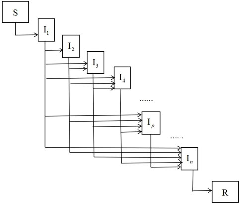
FIGURE 1. Disease transmission paths.

TABLE 1

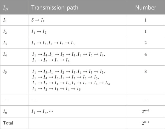
TABLE 1. Simulation parameter values for chapter 5.

Here, the next-generation method [38] is used to calculate the basic reproduction number. We rewrite system 1 as ($I_1,I_2,I_3,\cdots ,I_n,S,R$). It can be expressed as follows:

$r_i\left(x\right)=\left[\begin{array}{c}{\displaystyle \sum _{p=1}^n}{\beta }_{p}S{I}_p\\ 0\\ ⋮\\ 0\end{array}\right],h_i\left(x\right)=\left[\begin{array}{c}\left({\mu }_1+{\displaystyle \sum _{p=2}^n}{r}_p^1\right)I_1\\ -r_2^1{I}_1+\left({\mu }_2+{\displaystyle \sum _{p=3}^n}{r}_p^1\right)I_2\\ ⋮\\ -r_{n+1}^n{I}_n+\mu R\end{array}\right].$

$F$ and $V$ are the Jacobian matrices of $r_i\left(x\right)$ and $h_i\left(x\right)$. Then, we obtain

$F=\frac{\partial r_i}{\partial x_j}\left(x_0\right)=\left[\begin{array}{ccccccc}{\beta }_1\frac{\mathrm{\Lambda }}{\mu }& {\beta }_2\frac{\mathrm{\Lambda }}{\mu }& {\beta }_3\frac{\mathrm{\Lambda }}{\mu }& \cdots & {\beta }_n\frac{\mathrm{\Lambda }}{\mu }& 0& 0\\ 0& 0& 0& \cdots & 0& 0& 0\\ ⋮& ⋮& ⋮& \ddots & ⋮& ⋮& ⋮\\ 0& 0& 0& \cdots & 0& 0& 0\end{array}\right],$

$V=\frac{\partial h_i}{\partial x_j}\left(x_0\right)=\left[\begin{array}{cccccccc}{\mu }_1+{\displaystyle \sum _{p=2}^n}{r}_p^1& 0& 0& \cdots & 0& 0& 0& 0\\ -r_2^1& {\mu }_2+{\displaystyle \sum _{p=3}^n}{r}_p^2& 0& \cdots & 0& 0& 0& 0\\ -r_3^1& -r_3^2& {\mu }_3+{\displaystyle \sum _{p=4}^n}{r}_p^3& \cdots & 0& 0& 0& 0\\ ⋮& ⋮& ⋮& \ddots & ⋮& ⋮& ⋮& ⋮\\ -r_n^1& -r_n^2& -r_n^3& \cdots & -r_n^{n-1}& {\mu }_n+r_{n+1}^n& 0& 0\\ {\beta }_1\frac{\mathrm{\Lambda }}{\mu }& {\beta }_2\frac{\mathrm{\Lambda }}{\mu }& {\beta }_3\frac{\mathrm{\Lambda }}{\mu }& \cdots & {\beta }_{n-1}\frac{\mathrm{\Lambda }}{\mu }& {\beta }_n\frac{\mathrm{\Lambda }}{\mu }& \mu & 0\\ 0& 0& 0& \cdots & 0& r_n^{n-1}& 0& \mu \end{array}\right],$

where $1\le i,j\le n$. The basic reproduction number $R_0$ is the spectral radius of $F{V}^{-1}$. The elements of $F$ are all zero except these at the first row. So, we only need to consider the first column of $V^{-1}$. It is given by

$V^{-1}=\frac{\partial h_i}{\partial x_j}\left(x_0\right)=\left[\begin{array}{ccc}\frac{1}{A_1}& \cdots & \cdots \\ \frac{r_2^1}{A_1{A}_2}& \cdots & \cdots \\ \frac{r_2^1{r}_3^2+r_3^1{A}_2}{A_1{A}_2{A}_3}& \cdots & \cdots \\ ⋮& ⋮& ⋮\\ \frac{{\displaystyle \sum _{p=0}^{n-2}}{B}_{n-2}^p}{{\displaystyle \prod _{i=1}^n}{A}_i}& \cdots & \cdots \\ 0& ⋮& ⋮\\ 0& ⋮& ⋮\end{array}\right],A_i={\mu }_i+{\displaystyle \sum _{p=i+1}^n}{r}_p^1,i=\mathrm{1,2},\cdots ,n,$

where

$\begin{array}{l}{B}_{n-2}^0=r_n^1{\displaystyle \prod _{i=2}^n}{A}_i,\\ B_{n-2}^1={\displaystyle \sum _{p=2}^{n-1}}{r}_p^1{r}_n^p{\displaystyle \prod _{i=2}^{p-1}}{A}_i{\displaystyle \prod _{i=p+1}^{n-1}}{A}_i,\\ B_{n-2}^2={\displaystyle \sum _{p_1=2,p_2=3,p_2>p_1}^{n-1}}{r}_{p_1}^1{r}_{p_2}^{p_1}{r}_n^{p_2}{\displaystyle \prod _{i=2}^{p_1-1}}{A}_i{\displaystyle \prod _{i=p_1+1}^{p_2-1}}{A}_i{\displaystyle \prod _{i=p_2+1}^{n-1}}{A}_i,\\ B_{n-2}^3={\displaystyle \sum _{p_1=2,p_2=3,p_3=4,p_3>p_2>p_1}^{n-1}}{r}_{p_1}^1{r}_{p_2}^{p_1}{r}_{p_3}^{p_2}{r}_n^{p_3}{\displaystyle \prod _{i=2}^{p_1-1}}{A}_i{\displaystyle \prod _{i=p_1+1}^{p_2-1}}{A}_i{\displaystyle \prod _{i=p_2+1}^{p_3-1}}{A}_i{\displaystyle \prod _{i=p_3+1}^{n-1}}{A}_i,\\ \cdots \cdots ,\\ B_{n-2}^{n-2}={\displaystyle \prod _{i=1}^{i=n-1}}{r}_{i+1}^i.\end{array}$

Hence,

$F{V}^{-1}=\left[\begin{array}{ccc}{R}_{0\left(I_1\right)}+R_{0\left(I_2\right)}+R_{0\left(I_3\right)}+R_{0\left(I_4\right)}+\cdots +R_{0\left(I_n\right)}& \cdots & \cdots \\ 0& 0& 0\\ ⋮& ⋮& ⋮\\ 0& 0& 0\\ 0& 0& 0\end{array}\right],$

$R_0=\rho \left(F{V}^{-1}\right)=R_{0\left(I_1\right)}+R_{0\left(I_2\right)}+R_{0\left(I_3\right)}+R_{0\left(I_4\right)}+\cdots +R_{0\left(I_n\right)},$

where

$\begin{array}{l}{R}_{0\left(I_1\right)}={\beta }_1\frac{\mathrm{\Lambda }}{\mu }\frac{1}{A_1},\\ R_{0\left(I_2\right)}={\beta }_2\frac{\mathrm{\Lambda }}{\mu }\frac{r_2^1}{A_1{A}_2}={\beta }_2\frac{\mathrm{\Lambda }}{\mu }\frac{r_2^1}{A_1}\frac{1}{A_2},\\ R_{0\left(I_3\right)}={\beta }_3\frac{\mathrm{\Lambda }}{\mu }\frac{r_3^1{A}_2+r_2^1{r}_3^2}{A_1{A}_2{A}_3}={\beta }_3\frac{\mathrm{\Lambda }}{\mu }\left(\frac{r_3^1}{A_1}+\frac{r_2^1{r}_3^2}{A_1{A}_2}\right)\frac{1}{A_3},\\ R_{0\left(I_4\right)}={\beta }_4\frac{\mathrm{\Lambda }}{\mu }\frac{r_4^1{A}_2{A}_3+r_2^1{r}_4^2{A}_3+r_3^1{r}_4^3{A}_2+r_2^1{r}_3^2{r}_4^3}{A_1{A}_2{A}_3{A}_4}={\beta }_4\frac{\mathrm{\Lambda }}{\mu }\left(\frac{r_4^1}{A_1}+\frac{r_2^1{r}_4^2}{A_1{A}_2}+\frac{r_3^1{r}_4^3}{A_1{A}_3}+\frac{r_2^1{r}_3^2{r}_4^3}{A_1{A}_2{A}_3}\right)\frac{1}{A_4},\cdots \cdots ,\\ R_{0\left(I_n\right)}={\beta }_n\frac{\mathrm{\Lambda }}{\mu }\frac{C_{n-2}^0+C_{n-2}^1+\cdots +C_{n-2}^{n-2}}{{\displaystyle \prod _{i=1}^n}{A}_i}={\beta }_n\frac{\mathrm{\Lambda }}{\mu }\left(\frac{r_n^1}{A_1}+\frac{r_2^1{r}_n^2}{A_1{A}_2}+\cdots +\frac{r_2^1{r}_3^2{r}_n^3}{A_1{A}_2{A}_3}+\cdots +\frac{{\displaystyle \prod _{i=1}^{i=n-1}}{r}_{i+1}^i}{{\displaystyle \prod _{i=1}^{n-1}}{A}_i}\right)\frac{1}{A_n}.\end{array}$

Here, the basic reproduction number consists of $R_{0\left(I_i\right)}$ that is contributed by $I_i$. $A_i$ represents the elimination rate of infected population $I_i$, and $1/A_i$ can be seen as the illness period. It is found that $R_{0\left(I_i\right)}$ is equal to the product of infection rate, population size, and illness period. $I_1$ comes from 1 path $S\to I_1$. Its population size is $\mathrm{\Lambda }/\mu$. The infection and elimination rates are ${\beta }_1$ and $1/A_1$. $I_1$ contributes ${\beta }_1\mathrm{\Lambda }/\left(\mu A_1\right)$. $I_2$ comes from 1 path $I_1\to I_2$. Its population size is $\mathrm{\Lambda }{r}_2^1/\left(\mu A_1\right)$. The infection and elimination rates are ${\beta }_2$ and $1/A_2$. $I_2$ contributes ${\beta }_2\mathrm{\Lambda }{r}_2^1/\left(\mu A_1{A}_2\right)$. $I_3$ comes from 2 paths $I_1\to I_3,$ $I_1\to I_2\to I_3$. Its population size is from $I_1$ and $I_2$, which can be shown as $\mathrm{\Lambda }{r}_3^1/\left(\mu A_1\right)$ and $\mathrm{\Lambda }{r}_2^1{r}_3^2/\left(\mu A_1{A}_2\right)$. The infection and elimination rates are ${\beta }_3$ and $1/A_3$. So, $I_3$ contributes ${\beta }_3\mathrm{\Lambda }{r}_3^1/\left(\mu A_1{A}_3\right)+{\beta }_3\mathrm{\Lambda }{r}_2^1{r}_3^2/\left(\mu A_1{A}_2{A}_3\right)$. The contribution of $I_n$ can be obtained by analogy. Thus, we can get the basic reproduction number with very little calculations. We define this process as a path analysis method that can be applied for the bilinear compartment models. The key is to find out all transmission paths and different population sizes.

3 Application examples

For high-dimensional epidemic model, it is cumbersome and error-prone to derive the basic reproduction number using the next-generation method. In this section, we use the path analysis method of Section 2 to directly give the basic reproduction numbers for three bilinear compartment models without any calculation.

In [37], system (2) has two populations with infection capability, which are called asymptomatic $A\left(t\right)$ and infected $I\left(t\right)$ populations. $A\left(t\right)$ comes from the path $S\to A$, and $I\left(t\right)$ comes from the path $A\to I$. According to the path analysis method, the basic reproduction number can be expressed as $R_0=R_{0_A}+R_{0_I}$. The total population is $\left(\mu +\gamma \right)/\left(\mu +\nu +\gamma \right)$ through the first equation of the system. The population sizes of $A\left(t\right)$ and $I\left(t\right)$ are $\left(\mu +\gamma \right)/\left(\mu +\nu +\gamma \right)$ and $\alpha \left(\mu +\gamma \right)/\left[(\mu +\nu +\gamma \right)$ $\left.\left(\alpha +{\delta }_A+\mu \right)\right]$. The infection rates of $A\left(t\right)$ and $I\left(t\right)$ are ${\beta }_A$ and ${\beta }_I$. The elimination rates are $1/\left(\alpha +{\delta }_A+\mu \right)$ and $1/\left({\delta }_I+\mu \right)$. $A\left(t\right)$ and $I\left(t\right)$ contribute

$R_{0_A}={\beta }_A\frac{\mu +\gamma }{\mu +\nu +\gamma }\frac{1}{\alpha +{\delta }_A+\mu },R_{0_I}={\beta }_I\frac{\mu +\gamma }{\mu +\nu +\gamma }\frac{1}{{\delta }_I+\mu }.$

Therefore, the basic reproduction number is as follows:

$R_0={\beta }_A\frac{\mu +\gamma }{\mu +\nu +\gamma }\frac{1}{\alpha +{\delta }_A+\mu }+{\beta }_I\frac{\mu +\gamma }{\mu +\nu +\gamma }\frac{1}{{\delta }_I+\mu },$

$\left\{\begin{array}{l}\frac{dS\left(t\right)}{dt}=\mu -\left({\beta }_{A}A\left(t\right)+{\beta }_{I}I\left(t\right)\right)S\left(t\right)-\left(\mu +\nu \right)S\left(t\right)+\gamma R\left(t\right),\\ \frac{dA\left(t\right)}{dt}=\left({\beta }_{A}A\left(t\right)+{\beta }_{I}I\left(t\right)\right)S\left(t\right)-\left(\alpha +{\delta }_A+\mu \right)A\left(t\right),\\ \frac{dI\left(t\right)}{dt}=\alpha A\left(t\right)-\left({\delta }_I+\mu \right)I\left(t\right),\\ \frac{dR\left(t\right)}{dt}={\delta }_{A}A\left(t\right)+{\delta }_{I}I\left(t\right)+\nu S\left(t\right)-\left(\gamma +\mu \right)R\left(t\right).\end{array}\right.(2)$

System (3) with nine dimensions has been developed in [25] to depict the transmission of COVID-19. The first equation reveals that $I_{ss},I_{ms}$, and $I_a$ are infectious. $I_{ss},I_{ms}$, and $I_a$ come from the paths $S\to E\to I_{ss}$, $S\to E\to I_{ms}$, and $S\to E\to I_a$, respectively. So, the basic reproduction number can be

$\left\{\begin{array}{l}\frac{dS\left(t\right)}{dt}=-\beta \frac{S\left(t\right)}{N}\left(I_{ss}\left(t\right)+I_{ms}\left(t\right)+I_a\left(t\right)\right),\\ \frac{dE\left(t\right)}{dt}=\beta \frac{S\left(t\right)}{N}\left(I_{ss}\left(t\right)+I_{ms}\left(t\right)+I_a\left(t\right)\right)-kE\left(t\right),\\ \frac{d{I}_{ss}\left(t\right)}{dt}=k{p}_{1}E\left(t\right)-h{I}_{ss}\left(t\right),\\ \frac{d{I}_{ms}\left(t\right)}{dt}=k{p}_{2}E\left(t\right)-{\gamma }_3{I}_{ms}\left(t\right),\\ \frac{d{I}_a\left(t\right)}{dt}=k\left(1-p_1-p_2\right)E\left(t\right)-{\gamma }_3{I}_a\left(t\right),\\ \frac{dH\left(t\right)}{dt}=h{q}_1{I}_{ss}\left(t\right)-H\left(t\right),\\ \frac{d{I}_{cu}\left(t\right)}{dt}=h\left(1-q_1\right)I_{ss}\left(t\right)-I_{cu},\\ \frac{dR\left(t\right)}{dt}={\gamma }_3{I}_{ms}\left(t\right)+{\gamma }_3{I}_a\left(t\right)+\left(1-{\delta }_1\right)H\left(t\right)+\left(1-{\gamma }_1\right)I_{cu}\left(t\right),\\ \frac{dD\left(t\right)}{dt}={\delta }_{1}H\left(t\right)+{\gamma }_1{I}_{cu}\left(t\right),\end{array}\right.(3)$

shown as $R_0=R_{0_{I_{ss}}}+R_{0_{I_{ms}}}+R_{0_{I_a}}$. The infection rates of the three populations are $\beta$. The elimination rates of $I_{ss}$, $I_{ms}$, and $I_a$ are $1/h$, $1/{\gamma }_3$, and $1/{\gamma }_3$. The population sizes of $I_{ss}$, $I_{ms}$, and $I_a$ are $p_1$, $p_2$, and $1-p_1-p_2$. $I_{ss}$, $I_{ms}$, and $I_a$ contribute

$R_{0_{I_{ss}}}=\beta \frac{p_1}{h},R_{0_{I_{ms}}}=\beta \frac{p_2}{{\gamma }_3},R_{0_a}=\beta \frac{1-p_1-p_2}{{\gamma }_3}.$

The basic reproduction number is as follows:

$R_0=\beta \frac{p_1}{h}+\beta \frac{p_2}{{\gamma }_3}+\beta \frac{1-p_1-p_2}{{\gamma }_3},$

$\left\{\begin{array}{l}\frac{dS}{dt}=\mathrm{\Pi }-\frac{S\left(\beta I+r_Q\beta Q+r_A\beta A\right)+r_J\beta J}{N}-\mu S,\\ \frac{dE}{dt}=\frac{S\left(\beta I+r_Q\beta Q+r_A\beta A\right)+r_J\beta J}{N}-\left({\gamma }_1+k_1+\mu \right)E,\\ \frac{dQ}{dt}={\gamma }_{1}E-\left(k_2+{\sigma }_1+\mu \right)Q,\frac{dA}{dt}=p{k}_{1}E-\left({\sigma }_2+\mu \right)A,\\ \frac{dI}{dt}=\left(1-p\right)k_{1}E-\left({\gamma }_2+{\sigma }_3+\mu \right)I,\\ \frac{dJ}{dt}=k_{2}Q+{\gamma }_{2}I-\left(\delta +{\sigma }_4+\mu \right)J,\\ \frac{dR}{dt}={\sigma }_{1}Q+{\sigma }_{2}A+{\sigma }_{3}I+{\sigma }_{4}J-\mu R.\end{array}\right.(4)$

In [13], an epidemic model (4) incorporating quarantine was built to predict the COVID-19 trend in the United Kingdom. The first equation shows that the quarantine $Q\left(t\right)$, asymptomatic $A\left(t\right)$, symptomatic $I\left(t\right)$, and isolated $J\left(t\right)$ populations are infectious in this system. $Q\left(t\right)$, $A\left(t\right)$, and $I\left(t\right)$ come from the paths $S\to E\to Q$, $S\to E\to A$, and $S\to E\to I$. $J\left(t\right)$ is from two paths $S\to E\to Q\to J$ and $S\to E\to I\to J$. The basic reproduction number can be denoted as $R_0=R_{0_Q}+R_{0_A}+R_{0_I}+R_{0_{J_1}}+R_{0_{J_2}}$. The population sizes of $Q\left(t\right)$, $A\left(t\right)$, and $I\left(t\right)$ are 1. The population size of $J\left(t\right)$ can be divided into two parts. One part from $Q\left(t\right)$ is $k_2/\left(k_2+{\sigma }_1+\mu \right)$. The other part from $I\left(t\right)$ is ${\gamma }_2/\left({\gamma }_2+{\sigma }_3+\mu \right)$. The infection rates of $Q\left(t\right)$, $A\left(t\right)$, $I\left(t\right)$, and $J\left(t\right)$ are $r_Q\beta$, $r_A\beta$, $\beta$, and $r_J\beta$. The elimination rates are $\left.1/\left(k_2+{\sigma }_1+\mu \right.),1/\left({\sigma }_2+\mu \right.),1/\left({\gamma }_2+{\sigma }_3+\mu \right.\right)$ and $1/\left(\delta +{\sigma }_4+\mu \right)$. $Q\left(t\right)$, $A\left(t\right)$, $I\left(t\right)$, and $J\left(t\right)$ contribute

$R_{0_Q}=r_Q\beta \frac{1}{k_2+{\sigma }_1+\mu },R_{0_A}=r_A\beta \frac{1}{{\sigma }_2+\mu },R_{0_I}=\beta \frac{1}{{\gamma }_2+{\sigma }_3+\mu },$

$R_{0_J}=r_J\beta \frac{k_2}{k_2+{\sigma }_1+\mu }\frac{1}{\delta +{\sigma }_4+\mu }+r_J\beta \frac{{\gamma }_2}{{\gamma }_2+{\sigma }_3+\mu }\frac{1}{\delta +{\sigma }_4+\mu }.$

The basic reproduction number is

$\begin{array}{l}{R}_0=r_Q\beta \frac{1}{k_2+{\sigma }_1+\mu }+r_A\beta \frac{1}{{\sigma }_2+\mu }+\beta \frac{1}{{\gamma }_2+{\sigma }_3+\mu }\\ +r_J\beta \frac{k_2}{k_2+{\sigma }_1+\mu }\frac{1}{\delta +{\sigma }_4+\mu }+r_J\beta \frac{{\gamma }_2}{{\gamma }_2+{\sigma }_3+\mu }\frac{1}{\delta +{\sigma }_4+\mu }.\end{array}$

4 Global stability analysis

4.1 Global stability analysis of the disease-free equilibrium point

Theorem 4.1:. The disease-free equilibrium point of system (1) is $\left(\mathrm{\Lambda }/\mu ,\mathrm{0,0},\cdots ,0\right)$. It is globally stable if $R_0<1$.Proof. Let $I_i=R=0,i=\mathrm{1,2},\cdots ,n$. Then, we get $\left(\mathrm{\Lambda }/\mu ,\mathrm{0,0},\cdots ,0\right)$ as the disease-free equilibrium point. We define a linear function as follows:

$V={\displaystyle \sum _{i=1}^n}{m}_i{I}_i,$

where $m_q=\frac{{\displaystyle \sum _{p=0}^{n-q}}{\beta }_{q+p}\frac{\mathrm{\Lambda }}{\mu }{\displaystyle \prod _{i=q+p+1}^n}{A}_i{\displaystyle \prod _{i=q}^{q+p-1}}{r}_{i+1}^i}{{\displaystyle \prod _{i=q}^n}{A}_i}{r}_q^1$, $i=\mathrm{1,2},\cdots ,q,\cdots ,n$. Calculating the time derivative of $V$ along the solutions of system (1), we have

$\begin{array}{l}\frac{dV}{dt}=m_1\left[{\displaystyle \sum _{p=1}^n}{\alpha }_{p}S{I}_p-\left({\mu }_1+{\displaystyle \sum _{p=2}^n}{r}_p^1\right)I_1\right]+m_2\left[r_2^1{I}_1-\left({\mu }_2+{\displaystyle \sum _{p=3}^n}{r}_p^1\right)I_2\right]+\cdots +m_n\left[{\displaystyle \sum _{p=1}^{n-1}}{r}_n^p{I}_p-\left({\mu }_n+r_{n+1}^n\right)I_n\right],\\ \le \left(m_1{\beta }_1\frac{\mathrm{\Lambda }}{\mu }-m_1{A}_1+m_2{r}_2^1+m_3{r}_3^1+\cdots +m_n{r}_n^1\right)I_1,\\ =\left(\frac{{\beta }_1\frac{\mathrm{\Lambda }}{\mu }}{A_1}+\frac{m_2{r}_2^1}{A_1}+\frac{m_3{r}_3^1}{A_1}+\cdots +\frac{m_n{r}_n^1}{A_1}-1\right)A_1{I}_1,\\ =\left(\frac{{\beta }_1\frac{\mathrm{\Lambda }}{\mu }}{A_1}+\frac{{\displaystyle \sum _{i=2}^n}{m}_{2\left({\beta }_i\right)}{r}_2^1}{A_1}+\frac{{\displaystyle \sum _{i=3}^n}{m}_{3\left({\beta }_i\right)}{r}_3^1}{A_1}+\cdots +\frac{{\displaystyle \sum _{i=n}^n}{m}_{n\left({\beta }_i\right)}{r}_n^1}{A_1}-1\right)A_1{I}_1,\\ =\left(R_0-1\right)A_1{I}_1.\end{array}$

When $R_0<1$, $\frac{dV}{dt}<0$. According to Lyapunov’s second method [39–43], the disease-free equilibrium point is globally stable.

4.2 Global stability analysis of the endemic equilibrium point

Theorem 4.2:. When $R_0>1$, system (1) has an endemic equilibrium point, and it is globally stable.Proof. According to the equilibrium solution of system (1), we can arrive at

$\begin{array}{l}{I}_1=\frac{\mathrm{\Lambda }\left({\beta }_1+{\beta }_2{B}_2+{\beta }_3{B}_3+\cdots +{\beta }_n{B}_n\right)-\mu A_1}{A_1\left({\beta }_1+{\beta }_2{B}_2+{\beta }_3{B}_3+\cdots +{\beta }_n{B}_n\right)}>0,\\ \frac{\mathrm{\Lambda }\left({\beta }_1+{\beta }_2{B}_2+{\beta }_3{B}_3+\cdots +{\beta }_n{B}_n\right)}{\mu A_1}-1>0,\\ R_0-1>0.\end{array}$

Therefore, when $R_0>1$, system (1) has an endemic equilibrium point. The endemic equilibrium point can be represented as $\left(S^{*},I_1^{*},I_2^{*},\cdots ,I_n^{*},R^{*}\right)$. We define a Volterra-type Lyapunov function

$L\left(S,I_1,I_2,\cdots ,I_n\right)=m_0\left(S-S^{*}-S^{*}\ln \frac{S}{S^{*}}\right)+{\displaystyle \sum _{p=1}^n}{m}_p\left(I_p-I_p^{*}-I_p^{*}\ln \frac{I_p}{I_p^{*}}\right).$

We denote

$m_1=m_0,m_k=m_0\frac{{\beta }_k{S}^{*}{I}_k^{*}}{r_k^1{I}_1^{*}},k=\mathrm{2,3,4},\cdots ,n.$

Differentiating $L$ along system (1), we have

$\begin{array}{l}\frac{dL}{dt}\le m_0{\displaystyle \sum _{p=1}^n}{\beta }_p{S}^{*}{I}_p^{*}\left(1-\frac{S{I}_p}{S^{*}{I}_p^{*}}\right)\left(1-\frac{S^{*}}{S}\right)+m_0\mu S^{*}\left(1-\frac{S}{S^{*}}\right)\left(1-\frac{S^{*}}{S}\right)+m_1{\displaystyle \sum _{p=1}^n}\left({\beta }_p\frac{S{I}_p}{S^{*}{I}_p^{*}}-\frac{I_1}{I_1^{*}}\right)\left(1-\frac{I_1^{*}}{I_1}\right)\\ +\cdots \\ +m_q{\displaystyle \sum _{p=1}^{q-1}}{r}_q^p{I}_p^{*}\left(\frac{I_p}{I_p^{*}}-\frac{I_q}{I_q^{*}}\right)\left(1-\frac{I_q^{*}}{I_q}\right)+m_q{\displaystyle \sum _{p=q+1}^n}{t}_p{I}_p^{*}\left(\frac{I_p}{I_p^{*}}-\frac{I_q}{I_q^{*}}\right)\left(1-\frac{I_q^{*}}{I_q}\right)\\ +\cdots \\ +m_n{\displaystyle \sum _{p=1}^{n-1}}{r}_n^p{I}_p^{*}\left(\frac{I_p}{I_p^{*}}-\frac{I_n}{I_n^{*}}\right)\left(1-\frac{I_n^{*}}{I_n}\right).\end{array}$

By calculation, we can get

$\begin{array}{l}\frac{dL}{dt}\le m_0{\displaystyle \sum _{p=1}^n}{\beta }_n{S}^{*}{I}_n^{*}\left(1-\frac{S^{*}}{S}+\frac{I_n}{I_n^{*}}-\frac{S{I}_n}{S^{*}{I}_n^{*}}\right)+m_0\mu S^{*}\left(2-\frac{S}{S^{*}}-\frac{S^{*}}{S}\right)\\ +m_1{\beta }_1{S}^{*}{I}_1^{*}\left(1-\frac{S}{S^{*}}-\frac{I_1}{I_1^{*}}+\frac{S{I}_1}{S^{*}{I}_1^{*}}\right)+{\displaystyle \sum _{p=2}^n}{m}_1{\beta }_p{S}^{*}{I}_p^{*}\left(1-\frac{S{I}_1^{*}{I}_p}{S^{*}{I}_1{I}_p^{*}}-\frac{I_1}{I_1^{*}}+\frac{S{I}_p}{S^{*}{I}_p^{*}}\right)\\ +\cdots \\ +m_q{\displaystyle \sum _{p=1}^{q-1}}{r}_q^p{I}_p^{*}\left(1+\frac{I_p}{I_p^{*}}-\frac{I_q}{I_q^{*}}-\frac{I_p{I}_q^{*}}{I_p^{*}{I}_q}\right)+m_q{\displaystyle \sum _{p=q+1}^n}{t}_p{I}_p^{*}\left(1+\frac{I_p}{I_p^{*}}-\frac{I_q}{I_q^{*}}-\frac{I_p{I}_q^{*}}{I_p^{*}{I}_q}\right)\\ +\cdots \\ +m_n{\displaystyle \sum _{p=1}^{n-1}}{r}_n^p{I}_p^{*}\left(1+\frac{I_p}{I_p^{*}}-\frac{I_n}{I_n^{*}}-\frac{I_p{I}_n^{*}}{I_p^{*}{I}_n}\right).\end{array}$

Finally, we get

$\frac{dL}{dt}\le m_0{S}^{*}{I}_1^{*}\left(\mu +{\beta }_1\right)\left(2-\frac{S^{*}}{S}-\frac{S}{S^{*}}\right)+m_0{S}^{*}{\displaystyle \sum _{p=2}^n}{\beta }_p{I}_p^{*}\left(3-\frac{S^{*}}{S}-\frac{S{I}_1^{*}{I}_p}{S^{*}{I}_1{I}_p^{*}}-\frac{I_1{I}_p^{*}}{I_1^{*}{I}_p}\right)<0.$

According to Lyapunov’s second method, the endemic equilibrium point is globally stable.

5 Model simulation

We demonstrate the stabilities of the disease-free and endemic equilibrium points with 1, 2, 3, and 4 infected populations through simulations. Supplementary Material S1 gives the values of the parameters in different cases. When the infection rate $\alpha$ of $I_1$ is taken as 0.0001, 0.0002, and 0.0003, Figure 2A demonstrates the global stability of the disease-free equilibrium point with $R_0<1$. As it is taken as 0.0004, 0.0006, and 0.0008, Figure 2B demonstrates the global stability of the endemic equilibrium point with $R_0>1$. Figures 2C–F show the global stabilities of the equilibrium points with $n=2$. Figures 3, 4 show the conclusions with $n=\mathrm{3,4}$.

FIGURE 2

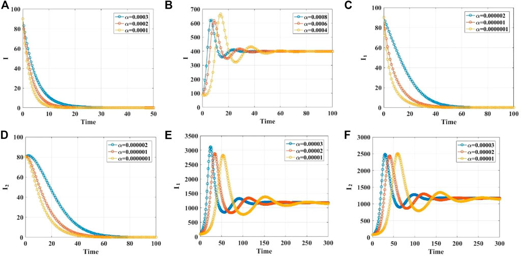
FIGURE 2. (A, B) The time series diagrams for $n=1$. (C–F) The time series diagrams for $n=2$.

FIGURE 3

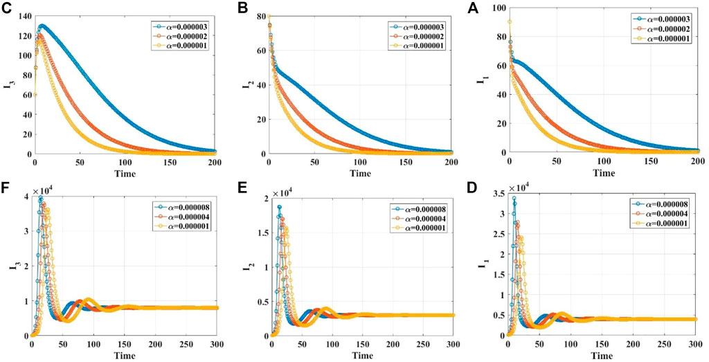
FIGURE 3. The time series diagrams for $n=3$.

FIGURE 4

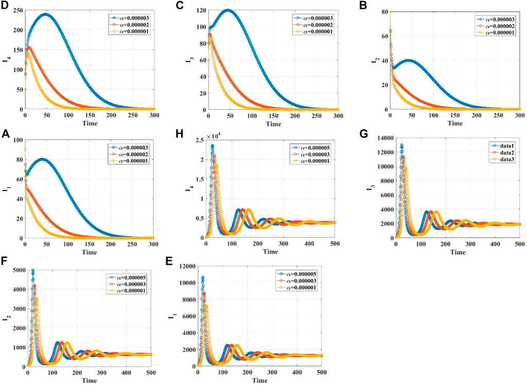
FIGURE 4. The time series diagrams for $n=4$.

6 Conclusion and discussions

This paper constructs a general epidemic system with bilinear incidence rates. It contains $n$ infected populations, where the first is the latent population. The transmission paths follow the top–down principle. We give all the disease transmission paths and find the number is equal to the sum of the combinatorial numbers. The basic reproduction number of our system has a reliable biological explanation and rigorous mathematical structure. It can be seen as the sum of the basic reproduction numbers of several infected populations with the ability to spread. We deform its structure and combine it with the disease transmission paths. A new method for calculating the basic reproduction number, the path analysis method, is proposed. The path analysis method is successfully applied to three representative examples containing different dimensions. Compared with the traditional next-generation method, the path analysis method greatly simplifies the calculation. It is possible to obtain the basic reproduction numbers of high-dimensional epidemic models without tedious calculations. The linear- and Volterra-type Lyapunov functions are used to prove the global stabilities of the disease-free and endemic equilibrium points. The global stability conditions are consistent with other studies. Simulations of the systems with 1, 2, 3, and 4 infected populations show that the infected populations converge to 0 when $R_0<1$ and to a constant when $R_0>1$. The path analysis method and the Volterra-type Lyapunov functions are not applicable to the systems with the nonlinear incidence rates, such as the Holling-type functions. For the simultaneous transmission of multiple infectious diseases, the path analysis method is also not feasible.

Data availability statement

The original contributions presented in the study are included in the article/Supplementary Material; further inquiries can be directed to the corresponding author.

Author contributions

YZ: conceptualization, methodology, software, and writing—original draft preparation. YD: visualization, investigation and supervision. MG: writing—reviewing and editing. All authors contributed to the article and approved the submitted version.

Funding

This work was supported by the National Natural Science Foundation of China (Grant No. 12271418).

Conflict of interest

The authors declare that the research was conducted in the absence of any commercial or financial relationships that could be construed as a potential conflict of interest.

Publisher’s note

All claims expressed in this article are solely those of the authors and do not necessarily represent those of their affiliated organizations, or those of the publisher, the editors, and the reviewers. Any product that may be evaluated in this article, or claim that may be made by its manufacturer, is not guaranteed or endorsed by the publisher.

Supplementary material

The Supplementary Material for this article can be found online at: https://www.frontiersin.org/articles/10.3389/fphy.2023.1158814/full#supplementary-material

References

1. Kermack WO, McKendrick AG. Contributions to the mathematical theory of epidemics. II.—the problem of endemicity[J]. Proc R Soc Lond Ser A, containing Pap a Math Phys character (1932) 138(834):55–83.

Google Scholar

2. Beretta E, Takeuchi Y. Global stability of an SIR epidemic model with time delays. J Math Biol (1995) 33(3):250–60. doi:10.1007/BF00169563

PubMed Abstract | CrossRef Full Text | Google Scholar

3. Korobeinikov A. Lyapunov functions and global stability for SIR and SIRS epidemiological models with non-linear transmission. Bull Math Biol (2006) 68:615–26. doi:10.1007/s11538-005-9037-9

PubMed Abstract | CrossRef Full Text | Google Scholar

4. Wei W, Xu W, Song Y, Liu J. Bifurcation and basin stability of an SIR epidemic model with limited medical resources and switching noise. Solitons & Fractals (2021) 152:111423. doi:10.1016/j.chaos.2021.111423

CrossRef Full Text | Google Scholar

5. Lei S, Jiang F, Su W, Chen C, Chen J, Mei W, et al. Clinical characteristics and outcomes of patients undergoing surgeries during the incubation period of COVID-19 infection. EClinicalMedicine (2020) 21:100331. doi:10.1016/j.eclinm.2020.100331

PubMed Abstract | CrossRef Full Text | Google Scholar

6. Chan-Yeung M, Xu RH. Sars: Epidemiology. Respirology (2003) 8:S9–S14. doi:10.1046/j.1440-1843.2003.00518.x

PubMed Abstract | CrossRef Full Text | Google Scholar

7. Eichner M, Dowell SF, Firese N. Incubation Period of Ebola hemorrhagic virus subtype zaire. Osong Public Health Res Perspect (2011) 2(1):3–7. doi:10.1016/j.phrp.2011.04.001

PubMed Abstract | CrossRef Full Text | Google Scholar

8. Schwartz IB, Smith HL. Infinite subharmonic bifurcation in an SEIR epidemic model. J Math Biol (1983) 18:233–53. doi:10.1007/bf00276090

PubMed Abstract | CrossRef Full Text | Google Scholar

9. Buonomo B, Lacitignola D. On the dynamics of an SEIR epidemic model with a convex incidence rate. Ricerche di matematica (2008) 57:261–81. doi:10.1007/s11587-008-0039-4

CrossRef Full Text | Google Scholar

10. Wang X, Tao Y, Song X. Pulse vaccination on SEIR epidemic model with nonlinear incidence rate. Appl Math Comput (2009) 210(2):398–404. doi:10.1016/j.amc.2009.01.004

CrossRef Full Text | Google Scholar

11. Efimov D, Ushirobira R. On an interval prediction of COVID-19 development based on a SEIR epidemic model. Annu Rev Control (2021) 51:477–87. doi:10.1016/j.arcontrol.2021.01.006

PubMed Abstract | CrossRef Full Text | Google Scholar

12. Wang L, Wang J, Zhao H, Shi YY, Wang K, Wu P, et al. Modelling and assessing the effects of medical resources on transmission of novel coronavirus (COVID-19) in Wuhan, China. Math Biosci Eng (2020) 17(4):2936–49. doi:10.3934/mbe.2020165

PubMed Abstract | CrossRef Full Text | Google Scholar

13. Nadim SS, Ghosh I, Chattopadhyay J. Short-term predictions and prevention strategies for COVID-19: A model-based study. Appl Math Comput (2021) 404:126251. doi:10.1016/j.amc.2021.126251

PubMed Abstract | CrossRef Full Text | Google Scholar

14. Das P, Nadim SS, Das S, et al. Dynamics of COVID-19 transmission with comorbidity: A data driven modelling based approach. Nonlinear Dyn (2021) 106:1197–211. doi:10.1007/s11071-021-06324-3

PubMed Abstract | CrossRef Full Text | Google Scholar

15. Péni T, Csutak B, Szederkényi G, Rost G. Nonlinear model predictive control with logic constraints for COVID-19 management. Nonlinear Dyn (2020) 102:1965–86. doi:10.1007/s11071-020-05980-1

PubMed Abstract | CrossRef Full Text | Google Scholar

16. Batabyal S, Batabyal A. Mathematical computations on epidemiology: A case study of the novel coronavirus (SARS-CoV-2). Theor Biosciences (2021) 140:123–38. doi:10.1007/s12064-021-00339-5

CrossRef Full Text | Google Scholar

17. Biswas SK, Ghosh JK, Sarkar S, Ghosh U. COVID-19 pandemic in India: A mathematical model study. Nonlinear Dyn (2020) 102:537–53. doi:10.1007/s11071-020-05958-z

PubMed Abstract | CrossRef Full Text | Google Scholar

18. Ojo MM, Peter OJ, Goufo EFD, Panigoro HS, Oguntolu FA. Mathematical model for control of tuberculosis epidemiology. J Appl Math Comput (2023) 69(1):69–87. doi:10.1007/s12190-022-01734-x

CrossRef Full Text | Google Scholar

19. Yin Q, Wang Z, Xia C, Bauch CT. Impact of co-evolution of negative vaccine-related information, vaccination behavior and epidemic spreading in multilayer networks. Commun Nonlinear Sci Numer Simulation (2022) 109:106312. doi:10.1016/j.cnsns.2022.106312

CrossRef Full Text | Google Scholar

20. Ojo MM, Peter OJ, Goufo EFD, Nisar KS. A mathematical model for the co-dynamics of COVID-19 and tuberculosis. Mathematics Comput Simulation (2023) 207:499–520. doi:10.1016/j.matcom.2023.01.014

CrossRef Full Text | Google Scholar

21. Fan J, Yin Q, Xia C, et al. Epidemics on multilayer simplicial complexes[J]. Proc R Soc A (2022) 478(2261):20220059.

CrossRef Full Text | Google Scholar

22. James Peter O, Ojo MM, Viriyapong R, Abiodun Oguntolu F. Mathematical model of measles transmission dynamics using real data from Nigeria. J Difference Equations Appl (2022) 28(6):753–70. doi:10.1080/10236198.2022.2079411

CrossRef Full Text | Google Scholar

23. Wang Z, Xia C, Chen Z, Chen G. Epidemic propagation with positive and negative preventive information in multiplex networks. IEEE Trans cybernetics (2020) 51(3):1454–62. doi:10.1109/TCYB.2019.2960605

CrossRef Full Text | Google Scholar

24. D'Arienzo M, Coniglio A. Assessment of the SARS-CoV-2 basic reproduction number, R0, based on the early phase of COVID-19 outbreak in Italy. Biosafety and health (2020) 2(2):57–9. doi:10.1016/j.bsheal.2020.03.004

PubMed Abstract | CrossRef Full Text | Google Scholar

25. Amouch M, Karim N. Modeling the dynamic of COVID-19 with different types of transmissions. J Chaos, Solitons Fractals (2021) 150:111188. doi:10.1016/j.chaos.2021.111188

CrossRef Full Text | Google Scholar

26. Ghosh JK, Biswas SK, Sarkar S, Ghosh U. Mathematical modelling of COVID-19: A case study of Italy. Math Comput Simulation (2022) 194:1–18. doi:10.1016/j.matcom.2021.11.008

CrossRef Full Text | Google Scholar

27. Lv R, Li H, Sun Q, et al. Stability analysis and optimal control of a time-delayed panic-spreading model[J]. Front Phys (2022) 1026.

Google Scholar

28. Zhang W, Ma X, Zhang Y, et al. Dynamical models of acute respiratory illness caused by human adenovirus on campus[J]. Front Phys (2022) 10:1325.

CrossRef Full Text | Google Scholar

29. Wang L, Jin Z, Wang H. A switching model for the impact of toxins on the spread of infectious diseases. J Math Biol (2018) 77:1093–115. doi:10.1007/s00285-018-1245-7

PubMed Abstract | CrossRef Full Text | Google Scholar

30. Wei F, Xue R. Stability and extinction of SEIR epidemic models with generalized nonlinear incidence. Math Comput Simulation (2020) 170:1–15. doi:10.1016/j.matcom.2018.09.029

CrossRef Full Text | Google Scholar

31. Pérez Á GC, Avila-Vales E, García-Almeida GE. Bifurcation analysis of an SIR model with logistic growth, nonlinear incidence, and saturated treatment. Complexity (2019) 2019:1–21. doi:10.1155/2019/9876013

CrossRef Full Text | Google Scholar

32. Peter OJ, Panigoro HS, Ibrahim MA, et al. Analysis and dynamics of measles with control strategies: A mathematical modeling approach[J]. Int J Dyn Control (2023) 1–15.

Google Scholar

33. Kammegne B, Oshinubi K, Babasola O, Peter OJ, Longe OB, Ogunrinde RB, et al. Mathematical modelling of the spatial distribution of a COVID-19 outbreak with vaccination using diffusion equation. Pathogens (2023) 12(1):88. doi:10.3390/pathogens12010088

PubMed Abstract | CrossRef Full Text | Google Scholar

34. Peter OJ, Yusuf A, Ojo MM, Kumar S, Kumari N, Oguntolu FA. A mathematical model analysis of meningitis with treatment and vaccination in fractional derivatives. Int J Appl Comput Math (2022) 8(3):117. doi:10.1007/s40819-022-01317-1

CrossRef Full Text | Google Scholar

35. Ojo MM, Benson TO, Peter OJ, Goufo EFD. Nonlinear optimal control strategies for a mathematical model of COVID-19 and influenza co-infection. Physica A: Stat Mech its Appl (2022) 607:128173. doi:10.1016/j.physa.2022.128173

CrossRef Full Text | Google Scholar

36. Melese AS, Makinde OD, Obsu LL. Mathematical modelling and analysis of coffee berry disease dynamics on a coffee farm. Math Biosciences Eng (2022) 19(7):7349–73. doi:10.3934/mbe.2022347

CrossRef Full Text | Google Scholar

37. Ottaviano S, Sensi M, Sottile S. Global stability of SAIRS epidemic models. Nonlinear Anal Real World Appl (2022) 65:103501. doi:10.1016/j.nonrwa.2021.103501

CrossRef Full Text | Google Scholar

38. Van den Driessche P, Watmough J. Reproduction numbers and sub-threshold endemic equilibria for compartmental models of disease transmission. Math biosciences (2002) 180(1-2):29–48. doi:10.1016/s0025-5564(02)00108-6

CrossRef Full Text | Google Scholar

39. Meskaf A, Khyar O, Danane J, Allali K. Global stability analysis of a two-strain epidemic model with non-monotone incidence rates. Solitons & Fractals (2020) 133:109647. doi:10.1016/j.chaos.2020.109647

CrossRef Full Text | Google Scholar

40. Safi MA, Garba SM. Global stability analysis of SEIR model with holling type II incidence function[J]. Comput Math Methods Med (2012) 2012.

PubMed Abstract | CrossRef Full Text | Google Scholar

41. Li CL, Cheng CY, Li CH. Global dynamics of two-strain epidemic model with single-strain vaccination in complex networks. Nonlinear Analysis: Real World Applications (2023) 69:103738. doi:10.1016/j.nonrwa.2022.103738

PubMed Abstract | CrossRef Full Text | Google Scholar

42. Khan Z A, Alaoui A L, Zeb A, Tilioua M, Djilali S. Global dynamics of a SEI epidemic model with immigration and generalized nonlinear incidence functional. Results in Physics (2021) 27:104477. doi:10.1016/j.rinp.2021.104477

CrossRef Full Text | Google Scholar

43. Saha S, Samanta G P, Nieto J J. Epidemic model of COVID-19 outbreak by inducing behavioural response in population. Nonlinear dynamics (2020) 102:455–87. Supplementary Material. doi:10.1007/s11071-020-05896-w

PubMed Abstract | CrossRef Full Text | Google Scholar