Original and modified non-perturbative renormalization group equations of the BMW scheme at the arbitrary order of truncation

1 Introduction

The renormalization group (RG) method is one of the most widely used approaches in the analysis of critical phenomena [1–5]. Here, we consider the non-perturbative RG approach [6–9], focusing on the Wetterich equation and its approximation schemes, developing further the research initiated in [10].

The functional renormalization group approach, which is at the heart of models such as the Wetterich and the Polchinski equations, provides an appropriate framework for the analysis of a range of central problems in many areas, including quantum systems, Yang–Mills theories, and statistical physics, see, e.g., [11], for a review. The Wetterich and Polchinski equations of the functional renormalization group belong to the so called non-perturbative RG equations. They have been successfully applied to many particular systems, including the Ginzburg–Landau model [10–18], quantum models and quantum gravity [19–30], and the tensorial group field theory [31]. It has been applied to equilibrium, as well as out-of-equilibrium systems and critical dynamics [32–34]. A recent review of all these applications is given in [35].

While the Wetterich equation itself is exact, it cannot be solved exactly. Approximate closed equations are obtained from it, applying certain truncation schemes for the effective action. The local potential approximation (LPA) is a widely known lowest-order approximation, which is traditionally improved step by step by the derivative expansion (DE) [9,14]. As alternative truncation schemes, the vertex expansion [14], the BMW scheme [17], and the recent scheme proposed in [10] can be mentioned. In distinction to the derivative expansion, which relies on the small momentum (wave vector magnitude) approximation, the latter two schemes preserve the full momentum dependence.

In this paper, we report the results of a significant further development of the BMW scheme for the scalar model, deriving explicit equations for calculations at the arbitrary order of truncation within this scheme, as well as proposing useful modifications of the original BMW scheme. Moreover, we established an intrinsic link between the equations of the BMW scheme and those of the recent scheme proposed in [10] at the first order of truncation. A recently developed method of semi-analytic approximations [36] was used to solve these equations.

The usefulness of our new developments is demonstrated in example calculations for the scalar model in three dimensions, where we evaluate the critical exponents, including the subleading correction-to-scaling exponent ω₂, for which quite limited results are available in the literature. Apparently, such results for ω₂ are obtained here for the first time from the Wetterich equation beyond the LPA, and we found only a relatively old estimate ω₂ = 1.67(11) from the Polchinski equation at the $O\left({\partial }^2\right)$ order of DE [37]. The RG estimations of the correction-to-scaling exponents have a fundamental significance as a crucial test of consistency with the conformal field theory (CFT) [38,39]. The RG estimate of ω₂ mentioned here does not reveal such a consistency, since ω₂ = 3.8956(43) is expected from the CFT [39,40]. We will return to this issue in the summary of our current results at the end of this paper.

Our paper is organized as follows. The Wetterich equation is reviewed in Sec. 2, and the BMW scheme of its truncation is reviewed in Sec. 3. Our new developments of the BMW scheme, including the equations at the arbitrary order of truncation, are presented in Sec. 4 with details of the derivation being given in Supplementary Material SA1. The comparison of equations of the BMW scheme with those derived in [10] is made in Sec. 5, providing the dimensionless form of these equations in Sec. 6. The results of numerical calculations are collected in Sec. 7. The summary of results and outlook, pointing to potential further applications and developments, are provided in Sec. 8.

2 Wetterich equation

In statistical physics, equilibrium systems of interacting particles are routinely described by the action S = H/(k_BT), where H is the Hamiltonian and k_B is the Boltzmann constant. A basic example is the Ising model with S [σ] = −β∑_⟨ij⟩σ_iσ_j − h∑_iσ_i, where σ_i = ±1 is the spin variable at the ith lattice site, ⟨ij⟩ denotes the pairs of nearest neighbors, β is the coupling constant, and h is the normalized (divided by k_BT) interaction energy between a spin with σ_i = ±1 and the external field. Another simple example is the φ⁴ model with $S[\phi ]=\int d^{d}x\left\{\alpha {\phi }^2+\beta {({\phi }^2)}^2+\gamma {(\nabla \phi )}^2\right\}$, where α, β and γ are the expansion coefficients for the density of S with a continuous order parameter φ(x), which depends on the coordinate x in the d-dimensional space. In the simplest case, it is scalar, but can also be an n-component vector. The scalar φ⁴ model is known to belong to the Ising universality class, which means that the behavior of φ⁴ and the Ising models near the phase transition point is described by the same critical exponents.

It is convenient to use the wave vector representation of the action S[φ] via the Fourier transformation φ(x) = Ω^−1/2 ∑_qφ(q)e^iqx, where Ω is the volume of the system. The critical behavior is related to the long-wavelength (infrared) or small-|q| fluctuations [3], but one should also control the ultraviolet fluctuations. A point here is that S[φ] might be ill-defined without an appropriate upper or ultraviolet cut-off in the wave vector (momentum) space. In the φ⁴ model, one needs to introduce such a cut-off, e.g., by setting φ(q) ≡ 0 at q > Λ (where q = |q|) to avoid ultraviolet divergences in various calculations, e.g., in the calculation of ⟨φ²⟩. The cut-off parameter Λ refers to the shortest or “microscopic” length scale ∼ π/Λ of the model, like the lattice constant in the Ising model.

The general idea of the RG method is to look at a system on different length scales. In the Wetterich functional RG approach [6,9], this idea is realized by introducing an infrared running cut-off scale k, in such a way that fluctuations with q ≲ k are suppressed, those with q ≫ k being practically unaffected. For this purpose, the action is modified as S[φ] → S[φ] + ΔS_k[φ] [9], where

$\mathrm{\Delta }{S}_k\left[\phi \right]=\frac{1}{2}\int \frac{d^{d}q}{{\left(2\pi \right)}^d}{\displaystyle \sum _{i=1}^N}{\phi }_i\left(-\mathbf{q}\right)R_k\left(q\right){\phi }_i\left(\mathbf{q}\right).(1)$

Here, φ is an N-component vector with components φ_i, whereas R_k(q) is the infrared cut-off function with properties R_k(q) → 0 at k → 0 and R_k(q) → ∞ at k → ∞ for fixed q. A simple choice, proposed in [6,9], is

$R_k\left(q\right)\sim \frac{q^2}{e^{q^2/k^2}-1}.(2)$

For q² ≪ k², this cut-off behaves as R_k(q) ∼ k². It means that the Fourier modes φ_i(q) with small momenta q < k acquire a weight factor or effective mass ∼ k included in the term (1). This additional mass acts as an effective infrared cut-off for these low-momentum modes. More precisely, this effect is essential in vicinity of the critical point, where R_k(q) smoothly cuts off the critical infrared fluctuations at a finite k. The cut-off function (2) tends (exponentially fast) to zero at large q/k values; therefore, the high-momentum modes with q/k → ∞ are not disturbed by ΔS_k[φ].

Further on, an averaged order parameter ϕ(x) = ⟨φ(x)⟩ is introduced, where the averaging is performed over φ(x) in the presence of external sources J(x). The averaged field ϕ(x) depends on J(x), and this dependence is affected by k, i.e., ϕ = ϕ_k(J). There exists also the inverse relation in the sense of the Legendre transformation J = J_k(ϕ). The effective average action Γ_k[ϕ] is considered as a functional of ϕ according to the definition

${\mathrm{\Gamma }}_k\left[\varphi \right]=-\ln {\mathcal{Z}}_k\left[J\right]+\int d^{d}x{\displaystyle \sum _i}{J}_i{\varphi }_i-\mathrm{\Delta }{S}_k\left[\varphi \right],(3)$

where J_i are the components of the vector J(x) and ${\mathcal{Z}}_k$ is the partition function

${\mathcal{Z}}_k\left[J\right]=\int D\phi \exp \left(-S\left[\phi \right]-\mathrm{\Delta }{S}_k\left[\phi \right]+\int d^{d}x{\displaystyle \sum _i}{J}_i{\phi }_i\right).(4)$

In (3), J(x) is the Legendre transform of ϕ(x), i.e., J = J_k(ϕ).

An exact RG flow equation, describing the variation of Γ_k[ϕ] with the infrared cut-off scale k, has been obtained in [6]. A detailed non-perturbative derivation has been later reported in [9]. This equation, called the Wetterich equation, reads

$\frac{\partial }{\partial k}{\mathrm{\Gamma }}_k\left[\varphi \right]=\frac{1}{2}\mathrm{T}\mathrm{r}\left\{{\left[{\mathrm{\Gamma }}_k^{\left(2\right)}\left[\varphi \right]+R_k\right]}^{-1}\frac{\partial }{\partial k}{R}_k\right\}.(5)$

In this equation, k decreases toward k = 0, starting from some initial value k₀. Thus, it generally allows describing the physics of various models with various choices of the order-parameter field by smoothly interpolating between different length scales.

Starting with k₀ = Λ (as in our calculations), only the fluctuations at the microscopic length scale q ∼Λ are properly taken into account in the initial stage of the integration of RG flow Eq. 5. Fluctuations of the original model (where ΔS_k = 0) with longer and longer wavelengths are gradually restored as k → 0. At k = 0, all fluctuation modes are included so that Γ_k=0 [ϕ] is the effective action of the original model, defined by (3) without the term ΔS_k [ϕ]. Another possibility, discussed in [35], is to choose k₀ ≫Λ. In this case, all fluctuations are frozen at the beginning (since the original model contains only the modes with q < Λ, and these are suppressed at k ≫Λ) and ${\mathrm{\Gamma }}_{k_0}[\varphi ]=S[\varphi ]$ holds as in Landau’s mean-field theory of phase transitions.

For the O(N) model, ϕ(x) is a vector with components ϕ_j(x), where j = 1, … , N. It is convenient to consider (5) in the space of wave vectors q, where

${\varphi }_j\left(\mathbf{x}\right)={\mathrm{\Omega }}^{-1/2}{\displaystyle \sum _{\mathbf{q}}}{\varphi }_j\left(\mathbf{q}\right)e^{i\mathbf{q}\mathbf{x}},(6)$

${\varphi }_j\left(\mathbf{q}\right)={\mathrm{\Omega }}^{-1/2}\int {\varphi }_j\left(\mathbf{x}\right)e^{-i\mathbf{q}\mathbf{x}}d\mathbf{x},(7)$

Ω being the volume of the system, for which periodic boundary conditions are assumed. The wave vectors are restricted by the upper cut-off, i.e., q < Λ. In this representation, the quantity ${\mathrm{\Gamma }}_k^{(2)}[\varphi ]$ is a matrix with elements

${\left({\mathrm{\Gamma }}_k^{\left(2\right)}\right)}_{ij}\left({\mathbf{q},\mathbf{q}}^{\prime }\right)=\frac{{\delta }^2{\mathrm{\Gamma }}_k\left[\varphi \right]}{\delta {\varphi }_i\left(-\mathbf{q}\right)\delta {\varphi }_j\left({\mathbf{q}}^{\prime }\right)}.(8)$

For the discrete wave vectors in (6), the cut-off function R_k is represented as [10]

$R_{k,ij}\left({\mathbf{q},\mathbf{q}}^{\prime }\right)=R_k\left(q\right){\delta }_{ij}{\delta }_{{\mathbf{q,q}}^{\prime }}.(9)$

The choice of R_k(q) is not unique, and several possibilities have been considered in [11,18]. For simplicity, here we have limited our choice to

$R_k\left(q\right)=\frac{\alpha Z_k{q}^2}{e^{q^2/k^2}-1},(10)$

traditionally used in many investigations [9,14,17], where Z_k is a renormalization constant and α is an optimization parameter. This cut-off function coincides with (2) and, thus, has the required properties discussed before. It allowed us to compare the results with those of [17], where the same cut-off function was used.

3 The BMW scheme of truncation

Here, we review the BMW truncation scheme for the scalar model, considered in detail in [17], noting that the N-component case has also been considered there in the Appendix. In the BMW truncation scheme, one considers the s-point functions ${\mathrm{\Gamma }}_k^{(s)}({\mathbf{q}}_1,{\mathbf{q}}_2,\dots ,{\mathbf{q}}_s;\varphi )$ as the Fourier transforms of δ^sΓ_k [ϕ]/(δϕ(x₁)δϕ(x₂)⋯δϕ(x_s)). We found it convenient to use an equivalent definition in the wave vector space, i.e.,

${\mathrm{\Gamma }}_k^{\left(s\right)}\left({\mathbf{q}}_1,{\mathbf{q}}_2,\dots ,{\mathbf{q}}_s;\varphi \right)={\mathrm{\Omega }}^{\frac{s}{2}-1}\frac{{\delta }^s{\mathrm{\Gamma }}_k\left[\varphi \right]}{\delta \varphi \left({\mathbf{q}}_1\right)\delta \varphi \left({\mathbf{q}}_2\right)\cdots \delta \varphi \left({\mathbf{q}}_s\right)},s\ge 2.(11)$

The basic idea of this truncation scheme is to consider first a hierarchy of exact equations for these s-point functions, obtained by applying the functional derivatives to (5). Approximate closed equations are then obtained, using certain approximations of the higher order functions (at orders s + 2 and s + 1) by the lower-order functions (up to the order s).

For constant ϕ, one has

${\mathrm{\Gamma }}_k\left[\varphi \right]=\mathrm{\Omega }{V}_k\left(\varphi \right),(12)$

where V_k(ϕ) is the potential. The exact RG flow equation for it is obtained by evaluating the Wetterich equation at ϕ = const. Using the notations t = ln k, $\rho =\frac{1}{2}{\varphi }^2$, and

${\int }_q\equiv \int \frac{d^{d}q}{{\left(2\pi \right)}^d},(13)$

where the integration is performed over the region q < Λ, this equation reads

${\partial }_t{V}_k\left(\rho \right)=\frac{1}{2}{\int }_q{\partial }_t{R}_k\left(q\right)G_k\left(\mathbf{q},\varphi \right),(14)$

where

$G_k^{-1}\left(\mathbf{q},\varphi \right)={\mathrm{\Gamma }}_k^{\left(2\right)}\left(q,\varphi \right)+R_k\left(q\right)(15)$

is the two-point correlation function with ${\mathrm{\Gamma }}_k^{(2)}(q,\varphi )\equiv {\mathrm{\Gamma }}_k^{(2)}(\mathbf{q},-\mathbf{q};\varphi )$, evaluated at ϕ = const.

In the zeroth-order approximation (s = 0) or LPA, one sets [17]

${\mathrm{\Gamma }}_k^{\left(2\right)}\left(q,\varphi \right)\to q^2+{\mathrm{\Gamma }}_k^{\left(2\right)}\left(0,\varphi \right)=q^2+{\partial }_{\varphi }^2{V}_k\left(\varphi \right),(16)$

where the coefficient 1 at q² corresponds to the usually assumed coefficient 1/2 at the gradient term (∇ϕ)² in the coordinate representation of Γ_k [ϕ], i.e.,

${\mathrm{\Gamma }}_k^{\text{LPA}}\left[\varphi \right]=\int d^{d}x\left\{\frac{1}{2}{\left(\nabla \varphi \right)}^2+V_k\left(\varphi \right)\right\}.(17)$

Using (16), Eq. 14 becomes a closed approximate RG flow equation for the potential V_k(ϕ).

In order to obtain the equations at the s = 2 order, one considers the RG flow for ${\mathrm{\Gamma }}_k^{(2)}$. An exact flow equation is obtained, taking two functional derivatives with respect to the field [based on (11)] in Wetterich Eq. 5 and evaluating the resulting expression at ϕ = const. It yields [17]

$\begin{array}{l}{\partial }_t{\mathrm{\Gamma }}_k^{\left(2\right)}\left(p,\varphi \right)={\int }_q{\partial }_t{R}_k\left(q\right)G_k^2\left(\mathbf{q},\varphi \right)\hfill \\ \hfill & \times \left\{{\mathrm{\Gamma }}_k^{\left(3\right)}\left(\mathbf{p},\mathbf{q},-\mathbf{p}-\mathbf{q};\varphi \right)G_k\left(\mathbf{q}+\mathbf{p},\varphi \right){\mathrm{\Gamma }}_k^{\left(3\right)}\left(-\mathbf{p},\mathbf{p}+\mathbf{q},-\mathbf{q};\varphi \right)-\frac{1}{2}{\mathrm{\Gamma }}_k^{\left(4\right)}\left(\mathbf{p},-\mathbf{p},\mathbf{q},-\mathbf{q};\varphi \right)\right\}.\hfill \end{array}(18)$

According to the original idea of the BMW truncation scheme, a closed approximate equation is obtained from this by setting the internal momenta equal to zero, i.e., q = 0, in the arguments of ${\mathrm{\Gamma }}_k^{(3)}$ and ${\mathrm{\Gamma }}_k^{(4)}$. Generally, this is done for ${\mathrm{\Gamma }}_k^{(s+1)}$ and ${\mathrm{\Gamma }}_k^{(s+2)}$ at order s. Thus, the momentum dependence of the highest-order functions is represented in a simplified approximate form, considering q as a small quantity. Using the exact formula

${\mathrm{\Gamma }}_k^{\left(s+1\right)}\left(\left\{{\mathbf{p}}_i\right\},\mathbf{0};\varphi \right)={\partial }_{\varphi }{\mathrm{\Gamma }}_k^{\left(s\right)}\left(\left\{{\mathbf{p}}_i\right\};\varphi \right)\text{for}\varphi =const,(19)$

these simplified expressions for ${\mathrm{\Gamma }}_k^{(s+1)}$ and ${\mathrm{\Gamma }}_k^{(s+2)}$ are further reduced to the derivatives of ${\mathrm{\Gamma }}_k^{(s)}$, thus obtaining closed equations. Equation 19 is a consequence of (11), noting that ϕ(q) = Ω^1/2ϕ δ_q,0 holds for homogeneous field ϕ(x) = ϕ = const according to (7).

At s = 2, the equation for ${\mathrm{\Gamma }}_k^{(2)}(p,\varphi )$ reads [17]

${\partial }_t{\mathrm{\Gamma }}_k^{\left(2\right)}=J_3\left(p,\varphi \right){\left({\partial }_{\varphi }{\mathrm{\Gamma }}_k^{\left(2\right)}\right)}^2-\frac{1}{2}{I}_2\left(\varphi \right){\partial }_{\varphi }^2{\mathrm{\Gamma }}_k^{\left(2\right)},(20)$

where

$J_n\left(p,\varphi \right)={\int }_q{\partial }_t{R}_k\left(q\right)G_k\left(\mathbf{p}+\mathbf{q},\varphi \right)G_k^{n-1}\left(\mathbf{q},\varphi \right),(21)$

$I_n\left(\varphi \right)=J_n\left(0,\varphi \right).(22)$

It is important to note that ${\mathrm{\Gamma }}_k^{(2)}$ is represented exactly as

${\mathrm{\Gamma }}_k^{\left(2\right)}\left(p,\varphi \right)={\mathrm{\Gamma }}_k^{\left(2\right)}\left(p,\varphi \right)-{\mathrm{\Gamma }}_k^{\left(2\right)}\left(0,\varphi \right)+{\partial }_{\varphi }^2{V}_k\left(\varphi \right),(23)$

keeping the term ${\partial }_{\varphi }^2{V}_k(\varphi )$, inherited from the zeroth-order approximation, untouched and solving the RG flow equation for the difference ${\mathrm{\Gamma }}_k^{(2)}(p,\varphi )-{\mathrm{\Gamma }}_k^{(2)}(0,\varphi )$. Moreover, it has also been suggested in [17] to separate the zeroth-order contribution q² from this difference.

4 Equations of the BMW scheme at the arbitrary order of truncation

4.1 Exact RG flow equations for the n-point functions

Here, we derive exact RG flow equations for the n-point function at any n, from which approximate closed equations at arbitrary truncation order s are then obtained, as described in Sec. 4.3. In the following, we summarize these equations, the details of the derivation being provided in Supplementary Material SA1. For brevity, we omitted ϕ in the list of arguments of the n-point functions ${\mathrm{\Gamma }}_k^{(n)}$, noting also that this argument is subsequently replaced by ρ = ϕ²/2 in our treatment. Thus, according to Supplementary Material SA1, for ϕ = const, we have

$\begin{array}{ll}\hfill {\partial }_t{\mathrm{\Gamma }}_k^{\left(n\right)}\left({\mathbf{p}}_1,{\mathbf{p}}_2,\dots ,{\mathbf{p}}_n\right)& =\frac{1}{2}{\displaystyle \sum _{M=1}^n}{\left(-1\right)}^M{\displaystyle \sum _{\begin{array}{c}\hfill m_1,m_2,\dots ,m_M\hfill \\ \hfill m_1+\cdots +m_M=n\hfill \end{array}}}{\displaystyle \sum _{{\left\{j_{\ell }\left(i\right)\right\}}_{m_1,\dots ,m_M}^n}}{\int }_q{\partial }_t{R}_k\left(q\right)\hfill \\ \hfill & \times G_k\left(\mathbf{q}\right){\displaystyle \prod _{i=1}^M}{\mathrm{\Gamma }}_k^{\left(2+m_i\right)}\left({\mathbf{p}}_{j_1\left(i\right)},{\mathbf{p}}_{j_2\left(i\right)},\dots ,{\mathbf{p}}_{j_{m_i}\left(i\right)},{\stackrel{`}{\mathbf{Q}}}_i,{\mathbf{Q}}_i\right){\widehat{G}}_k\left({\mathbf{Q}}_i\right),\hfill \end{array}(24)$

where ${\sum }_{l=1}^n{\mathbf{p}}_l=\mathbf{0}$ holds, 1 ≤ m_i ≤ n are integers, and ${\left\{j_{\ell }(i)\right\}}_{m_1,\dots ,m_M}^n$ are the distributions of n integer numbers 1, 2, … , n over M boxes with m₁ numbers in the first box, m₂ numbers in the second box, and so on (totally n!/(m₁!m₂!⋯m_M!) possibilities). Here, j_ℓ(i) with ℓ = 1, 2, … , m_i are the numbers in the ith box. We ordered them by index ℓ in such a way that $j_1(i)<j_2(i)<\dots <j_{m_i}(i)$. In addition, ${\widehat{G}}_k(\mathbf{Q})$ is the correlation function, which is modified by the upper cut-off as

${\widehat{G}}_k\left(\mathbf{Q}\right)=G_k\left(\mathbf{Q}\right)\theta \left(\mathrm{\Lambda }-Q\right).(25)$

This cut-off is included here to follow a formal rigor in treating such cases, where the original action S[φ] is ill-defined without it, see Sec. 2. It influences the RG flow in the Wetterich equation only at k ∼Λ for k ≤ Λ. Therefore, it can be further omitted, considering the vicinity of the fixed point at k → 0, as it is usually performed in the literature.

For any given m₁, m₂, … m_M at the considered n, the wave vectors Q_i are defined by

${\stackrel{`}{\mathbf{Q}}}_i=-\mathbf{q}-{\displaystyle \sum _{l=i}^M}{\mathbf{P}}_l,1\le i\le M,(26)$

${\mathbf{Q}}_i=\mathbf{q}+{\displaystyle \sum _{l=i+1}^M}{\mathbf{P}}_l,1\le i\le M,(27)$

where the latter sum is defined as zero for i = M (so that Q_M = q) and

${\mathbf{P}}_i={\displaystyle \sum _{\ell =1}^{m_i}}{\mathbf{p}}_{j_{\ell }\left(i\right)},1\le i\le M.(28)$

At i = 1, Eqs 26, 27 reduce to

${\stackrel{`}{\mathbf{Q}}}_1=-\mathbf{q},{\mathbf{Q}}_1=\mathbf{q}-{\mathbf{P}}_1,(29)$

noting that

${\displaystyle \sum _{i=1}^M}{\mathbf{P}}_i={\displaystyle \sum _{l=1}^n}{\mathbf{p}}_l=\mathbf{0}.(30)$

The known Eq. 18 can be easily recovered from (24). Following notations introduced after Eq. 15 and noting that p₁ + p₂ = 0 holds in (24) at n = 2, we have ${\partial }_t{\mathrm{\Gamma }}_k^{(2)}(p_1)$ on the left-hand side of this equation at n = 2. In this case, the sum over M contains only two terms, M = 1 and M = 2. At M = 1, the next sum reduces to m₁ = n = 2, and the last sum reduces to j₁(1) = 1 and j₂(1) = 2. It corresponds to two numbers, 1 and 2, put in a single box (i = 1, ℓ = 1, 2). These numbers are identified with j₁(1) and j₂(1). One has j₁(1) = 1, j₂(1) = 2 due to the ordering j₁(1) < j₂(1). Furthermore, we find Q₁ = q from (27), P₁ = p₁ + p₂ = 0 from (28), and ${\stackrel{`}{\mathbf{Q}}}_1=-\mathbf{q}$ from (26). Hence, M = 1 gives the contribution

${\left({\partial }_t{\mathrm{\Gamma }}_k^{\left(2\right)}\left(p_1\right)\right)}_1=-\frac{1}{2}{\int }_q{\partial }_t{R}_k{G}_k^2\left(\mathbf{q}\right){\mathrm{\Gamma }}_k^{\left(4\right)}\left({\mathbf{p}}_1,-{\mathbf{p}}_1,-\mathbf{q},\mathbf{q}\right)(31)$

to (24), noting that ${\widehat{G}}_k(\mathbf{q})=G_k(\mathbf{q})$ holds, since 0 < q < Λ.

At M = 2, the second sum reduces to m₁ = m₂ = 1 for n = 2, whereas the following sum comprises two cases: 1) j₁(1) = 1, j₁(2) = 2 and 2) j₁(1) = 2, j₁(2) = 1 (we have i = 1, 2 and ℓ = 1). In the first case, we obtain (using Eqs 26–28, where p₁ + p₂ = 0) P₁ = p₁, P₂ = p₂, ${\stackrel{`}{\mathbf{Q}}}_1=-\mathbf{q}$, Q<sub>1</sub> = q + p<sub>2</sub>, ${\stackrel{`}{\mathbf{Q}}}_2=-\mathbf{q}-{\mathbf{p}}_2$, and Q₂ = q. The second symmetric case is obtained from the first one via p₁ ↔p₂. Hence, M = 2 gives the contribution

$\begin{array}{ll}\hfill {\left({\partial }_t{\mathrm{\Gamma }}_k^{\left(2\right)}\left(p_1\right)\right)}_2& =\frac{1}{2}{\int }_q{\partial }_t{R}_k\left(q\right)G_k^2\left(\mathbf{q}\right)\left[{\mathrm{\Gamma }}_k^{\left(3\right)}\left({\mathbf{p}}_1,-\mathbf{q},\mathbf{q}+{\mathbf{p}}_2\right){\widehat{G}}_k\left(\mathbf{q}+{\mathbf{p}}_2\right){\mathrm{\Gamma }}_k^{\left(3\right)}\left({\mathbf{p}}_2,-\mathbf{q}-{\mathbf{p}}_2,\mathbf{q}\right)\right.\hfill \\ \hfill & +{\mathrm{\Gamma }}_k^{\left(3\right)}\left({\mathbf{p}}_2,-\mathbf{q},\mathbf{q}+{\mathbf{p}}_1\right){\widehat{G}}_k\left(\mathbf{q}+{\mathbf{p}}_1\right){\mathrm{\Gamma }}_k^{\left(3\right)}\left({\mathbf{p}}_1,-\mathbf{q}-{\mathbf{p}}_1,\mathbf{q}\right)],\hfill \end{array}(32)$

where ${\widehat{G}}_k(\mathbf{q})=G_k(\mathbf{q})$ is used as in (31). This expression is modified by setting p₂ = −p₁. Furthermore, the replacement q → −q is performed in the first line of (32) (owing to the symmetric integration region |q| < Λ) followed by the change of the sign for the arguments of G_k and ${\widehat{G}}_k$ (since G_k(Q) = G_k (−Q)). In the second line of (32), the last two arguments of ${\mathrm{\Gamma }}_k^{(3)}$ are exchanged, using the symmetry of the n-point functions. After these replacements, it becomes evident that two terms in the square brackets give equal contributions, and (32) reduces to

${\left({\partial }_t{\mathrm{\Gamma }}_k^{\left(2\right)}\left(p_1\right)\right)}_2={\int }_q{\partial }_t{R}_k\left(q\right)G_k^2\left(\mathbf{q}\right){\mathrm{\Gamma }}_k^{\left(3\right)}\left({\mathbf{p}}_1,\mathbf{q},-\mathbf{q}-{\mathbf{p}}_1\right){\widehat{G}}_k\left(\mathbf{q}+{\mathbf{p}}_1\right){\mathrm{\Gamma }}_k^{\left(3\right)}\left(-{\mathbf{p}}_1,\mathbf{q}+{\mathbf{p}}_1,-\mathbf{q}\right).(33)$

Equation 18 is obtained by summing up both contributions (31) and (33), exchanging the last two arguments of ${\mathrm{\Gamma }}_k^{(4)}$ (using the symmetry), omitting the upper cut-off for ${\widehat{G}}_k(\mathbf{q}+{\mathbf{p}}_1)$, redenoting p₁ → p, and reintroducing the argument ϕ, which is skipped for brevity.

If ${\mathrm{\Gamma }}_k^{(n)}$ is an analytic function of ϕ² for even n, then it is representable as ϕ multiplied by an analytic function of ϕ² for odd n, as it follows from (19). Therefore, we introduce the new n-point functions

${\widehat{\mathrm{\Gamma }}}_k^{\left(n\right)}\stackrel{\mathrm{D}\mathrm{e}\mathrm{f}}{=}\left\{\begin{array}{c}{\mathrm{\Gamma }}_k^{\left(n\right)},\text{for\hspace{0.17em}even}n,\hfill \\ {\varphi }^{-1}{\mathrm{\Gamma }}_k^{\left(n\right)},\text{for\hspace{0.17em}odd}n,\hfill \end{array}\right.(34)$

which are all analytic functions of ρ = ϕ²/2. Substituting these new functions in RG flow Eq. 24, we easily obtain

$\begin{array}{ll}\hfill & {\partial }_t{\widehat{\mathrm{\Gamma }}}_k^{\left(n\right)}\left({\mathbf{p}}_1,{\mathbf{p}}_2,\dots ,{\mathbf{p}}_n\right)=\frac{1}{2}{\displaystyle \sum _{M=1}^n}{\left(-1\right)}^M{\displaystyle \sum _{\begin{array}{c}\hfill m_1,m_2,\dots ,m_M\hfill \\ \hfill m_1+\cdots +m_M=n\hfill \end{array}}}{\displaystyle \sum _{{\left\{j_{\ell }\left(i\right)\right\}}_{m_1,\dots ,m_M}^n}}{\int }_q{\partial }_t{R}_k\left(q\right)\hfill \\ \hfill & \times {\left(2\rho \right)}^{{\mu }_n\left(m_1,\dots ,m_M\right)}{G}_k\left(\mathbf{q}\right){\displaystyle \prod _{i=1}^M}{\widehat{\mathrm{\Gamma }}}_k^{\left(2+m_i\right)}\left({\mathbf{p}}_{j_1\left(i\right)},{\mathbf{p}}_{j_2\left(i\right)},\dots ,{\mathbf{p}}_{j_{m_i}\left(i\right)},{\stackrel{`}{\mathbf{Q}}}_i,{\mathbf{Q}}_i\right){\widehat{G}}_k\left({\mathbf{Q}}_i\right),\hfill \end{array}(35)$

where

${\mu }_n\left(m_1,\dots ,m_M\right)=\left\{\begin{array}{c}\mathcal{N}\left(m_1,\dots ,m_M\right)/2\text{for\hspace{0.17em}even}n,\hfill \\ \left(\mathcal{N}\left(m_1,\dots ,m_M\right)-1\right)/2\text{for\hspace{0.17em}odd}n,\hfill \end{array}\right.(36)$

where $\mathcal{N}(m_1,\dots ,m_M)$ is the number of odd m_i in the sequence m₁, m₂, … , m_M. Due to the condition m₁ + m₂ + ⋯ + m_M = n, $\mathcal{N}$ is even for even n and odd for odd n. Consequently, μ_n is always a non-negative integer number.

4.2 Some useful relations

In this section, we introduce some exact relations, which are useful for building up the approximation schemes in Sec. 4.3.

First, we consider the structure of arguments of the highest-order term ${\mathrm{\Gamma }}_k^{(n+2)}$ in Eq. 24 for ${\mathrm{\Gamma }}_k^{(n)}$. This term appears only at M = 1, m₁ = n, and there is only one $\left\{j_{\ell }(i)\right\}$ distribution possible in this case, i.e., i = 1, j_ℓ(1) = ℓ with 1 ≤ ℓ ≤ n. Since i = 1, we have Q₁ = q and ${\grave{\mathbf{Q}}}_1=-\mathbf{q}$ according to (29), noting that P₁ = p₁ + ⋯ + p_n = 0 holds for this $\left\{j_{\ell }(i)\right\}$. Thus, Eq. 24 contains ${\mathrm{\Gamma }}_k^{(n+2)}$ in the form of ${\mathrm{\Gamma }}_k^{(n+2)}({\mathbf{p}}_1,{\mathbf{p}}_2,\dots ,{\mathbf{p}}_n,-\mathbf{q},\mathbf{q})$.

Similarly, we consider the arguments of the ${\mathrm{\Gamma }}_k^{(n+1)}$ function, contained in the equation for ${\mathrm{\Gamma }}_k^{(n)}$. The (n + 1)-point function appears at M = 2 in two subcases: 1) m₁ = 1, m₂ = n − 1 and 2) m₁ = n − 1, m₂ = 1. Using relations (26)–(29), we easily establish that ${\mathrm{\Gamma }}_k^{(n+1)}$ is contained in the forms of ${\mathrm{\Gamma }}_k^{(n+1)}\left({\mathbf{p}}_{j_1},{\mathbf{p}}_{j_2},\dots ,{\mathbf{p}}_{j_{n-1}},-\mathbf{q}-{\sum }_{\ell =1}^{n-1}{\mathbf{p}}_{j_{\ell }},\mathbf{q}\right)$ and ${\mathrm{\Gamma }}_k^{(n+1)}\left({\mathbf{p}}_{j_1},{\mathbf{p}}_{j_2},\dots ,{\mathbf{p}}_{j_{n-1}},-\mathbf{q},\mathbf{q}-{\sum }_{\ell =1}^{n-1}{\mathbf{p}}_{j_{\ell }}\right)$, where all possible sequences of indices $\left\{j_{\ell }\right\}$ appear, which are obtained by skipping one of the numbers in the sequence 1, 2, … , n.

As the next step, we consider the exact relations

$\begin{array}{ll}\hfill & {\mathrm{\Gamma }}_k^{\left(n+2\right)}\left({\mathbf{p}}_1,{\mathbf{p}}_2,\dots ,{\mathbf{p}}_n,-\mathbf{q},\mathbf{q}\right)={\partial }_{\varphi }^2{\mathrm{\Gamma }}_k^{\left(n\right)}\left({\mathbf{p}}_1,{\mathbf{p}}_2,\dots ,{\mathbf{p}}_n\right)\hfill \\ \hfill & +{\mathrm{\Delta }}_{2,k}^{\left(n+2\right)}\left({\mathbf{p}}_1,{\mathbf{p}}_2,\dots ,{\mathbf{p}}_n,-\mathbf{q},\mathbf{q}\right),\hfill \end{array}(37)$

$\begin{array}{ll}\hfill & {\mathrm{\Gamma }}_k^{\left(n+1\right)}\left({\mathbf{p}}_{j_1},{\mathbf{p}}_{j_2},\dots ,{\mathbf{p}}_{j_{n-1}},-\mathbf{q}-\sum {\mathbf{p}}_{j_{\ell }},\mathbf{q}\right)\hfill \\ \hfill & ={\partial }_{\varphi }{\mathrm{\Gamma }}_k^{\left(n\right)}\left({\mathbf{p}}_{j_1},{\mathbf{p}}_{j_2},\dots ,{\mathbf{p}}_{j_{n-1}},-\sum {\mathbf{p}}_{j_{\ell }}\right)\hfill \end{array}(38)$

$+{\mathrm{\Delta }}_{1,k}^{\left(n+1\right)}\left({\mathbf{p}}_{j_1},{\mathbf{p}}_{j_2},\dots ,{\mathbf{p}}_{j_{n-1}},-\mathbf{q}-\sum {\mathbf{p}}_{j_{\ell }},\mathbf{q}\right),(\mathrm{})$

following from (19), where $\sum {\mathbf{p}}_{j_{\ell }}\equiv {\sum }_{\ell =1}^{n-1}{\mathbf{p}}_{j_{\ell }}$ and

$\begin{array}{ll}\hfill & {\mathrm{\Delta }}_{2,k}^{\left(n+2\right)}\left({\mathbf{p}}_1,{\mathbf{p}}_2,\dots ,{\mathbf{p}}_n,-\mathbf{q},\mathbf{q}\right)\stackrel{\mathrm{D}\mathrm{e}\mathrm{f}}{=}{\mathrm{\Gamma }}_k^{\left(n+2\right)}\left({\mathbf{p}}_1,{\mathbf{p}}_2,\dots ,{\mathbf{p}}_n,-\mathbf{q},\mathbf{q}\right)\hfill \\ \hfill & -{\mathrm{\Gamma }}_k^{\left(n+2\right)}\left({\mathbf{p}}_1,{\mathbf{p}}_2,\dots ,{\mathbf{p}}_n,\mathbf{0},\mathbf{0}\right),\hfill \end{array}(39)$

$\begin{array}{ll}\hfill & {\mathrm{\Delta }}_{1,k}^{\left(n+1\right)}\left({\mathbf{p}}_{j_1},{\mathbf{p}}_{j_2},\dots ,{\mathbf{p}}_{j_{n-1}},-\mathbf{q}-\sum {\mathbf{p}}_{j_{\ell }},\mathbf{q}\right)\hfill \\ \hfill & \stackrel{\mathrm{D}\mathrm{e}\mathrm{f}}{=}{\mathrm{\Gamma }}_k^{\left(n+1\right)}\left({\mathbf{p}}_{j_1},{\mathbf{p}}_{j_2},\dots ,{\mathbf{p}}_{j_{n-1}},-\mathbf{q}-\sum {\mathbf{p}}_{j_{\ell }},\mathbf{q}\right)\hfill \end{array}(40)$

$-{\mathrm{\Gamma }}_k^{\left(n+1\right)}\left({\mathbf{p}}_{j_1},{\mathbf{p}}_{j_2},\dots ,{\mathbf{p}}_{j_{n-1}},-\sum {\mathbf{p}}_{j_{\ell }},\mathbf{0}\right).(\mathrm{})$

Using these relations, ${\mathrm{\Gamma }}_k^{(n+1)}$ and ${\mathrm{\Gamma }}_k^{(n+2)}$ can be expressed by ${\partial }_{\varphi }{\mathrm{\Gamma }}_k^{(n)}$, ${\partial }_{\varphi }^2{\mathrm{\Gamma }}_k^{(n)}$, ${\mathrm{\Delta }}_{1,k}^{(n+1)}$, and ${\mathrm{\Delta }}_{2,k}^{(n+2)}$ in the equation for ${\mathrm{\Gamma }}_k^{(n)}$, noting that (38) holds for arbitrary wave vectors, and the arguments can be exchanged. In particular, one can exchange the last two arguments and replace q → −q to obtain the necessary relation for ${\mathrm{\Gamma }}_k^{(n+1)}\left({\mathbf{p}}_{j_1},{\mathbf{p}}_{j_2},\dots ,{\mathbf{p}}_{j_{n-1}},-\mathbf{q},\mathbf{q}-{\sum }_{\ell =1}^{n-1}{\mathbf{p}}_{j_{\ell }}\right)$.

In the following, we derive such relations for the n-point functions ${\widehat{\mathrm{\Gamma }}}_k^{(n+2)}$ and ${\widehat{\mathrm{\Gamma }}}_k^{(n+1)}$, expressed by the derivatives with respect to ρ. Using the definitions (34) and ρ = ϕ²/2, we obtain from (37) to (38) the desired equations:

$\begin{array}{ll}\hfill & {\widehat{\mathrm{\Gamma }}}_k^{\left(n+2\right)}\left({\mathbf{p}}_1,{\mathbf{p}}_2,\dots ,{\mathbf{p}}_n,-\mathbf{q},\mathbf{q}\right)=H_2^{\left(n\right)}{\widehat{\mathrm{\Gamma }}}_k^{\left(n\right)}\left({\mathbf{p}}_1,{\mathbf{p}}_2,\dots ,{\mathbf{p}}_n\right)\hfill \\ \hfill & +{\widehat{\mathrm{\Delta }}}_{2,k}^{\left(n+2\right)}\left({\mathbf{p}}_1,{\mathbf{p}}_2,\dots ,{\mathbf{p}}_n,-\mathbf{q},\mathbf{q}\right),\hfill \end{array}(41)$

$\begin{array}{ll}\hfill & {\widehat{\mathrm{\Gamma }}}_k^{\left(n+1\right)}\left({\mathbf{p}}_{j_1},{\mathbf{p}}_{j_2},\dots ,{\mathbf{p}}_{j_{n-1}},-\mathbf{q}-\sum {\mathbf{p}}_{j_{\ell }},\mathbf{q}\right)\hfill \\ \hfill & =H_1^{\left(n\right)}{\widehat{\mathrm{\Gamma }}}_k^{\left(n\right)}\left({\mathbf{p}}_{j_1},{\mathbf{p}}_{j_2},\dots ,{\mathbf{p}}_{j_{n-1}},-\sum {\mathbf{p}}_{j_{\ell }}\right)\hfill \end{array}(42)$

$+{\widehat{\mathrm{\Delta }}}_{1,k}^{\left(n+1\right)}\left({\mathbf{p}}_{j_1},{\mathbf{p}}_{j_2},\dots ,{\mathbf{p}}_{j_{n-1}},-\mathbf{q}-\sum {\mathbf{p}}_{j_{\ell }},\mathbf{q}\right),(\mathrm{})$

where $H_1^{(n)}$ and $H_2^{(n)}$ are the differential operators

$H_1^{\left(n\right)}=\left\{\begin{array}{c}{\partial }_{\rho }\text{for\hspace{0.17em}even}n\hfill \\ 1+2\rho {\partial }_{\rho }\text{for\hspace{0.17em}odd}n\hfill \end{array}\right.,(43)$

$H_2^{\left(n\right)}=\left\{\begin{array}{c}{\partial }_{\rho }+2\rho {\partial }_{\rho }^2\text{for\hspace{0.17em}even}n\hfill \\ 3{\partial }_{\rho }+2\rho {\partial }_{\rho }^2\text{for\hspace{0.17em}odd}n\hfill \end{array}\right.(44)$

and the quantities ${\widehat{\mathrm{\Delta }}}_{j,k}^{(n+i)}$ are defined as

$\begin{array}{ll}\hfill & {\widehat{\mathrm{\Delta }}}_{2,k}^{\left(n+2\right)}\left({\mathbf{p}}_1,{\mathbf{p}}_2,\dots ,{\mathbf{p}}_n,-\mathbf{q},\mathbf{q}\right)\stackrel{\mathrm{D}\mathrm{e}\mathrm{f}}{=}{\widehat{\mathrm{\Gamma }}}_k^{\left(n+2\right)}\left({\mathbf{p}}_1,{\mathbf{p}}_2,\dots ,{\mathbf{p}}_n,-\mathbf{q},\mathbf{q}\right)\hfill \\ \hfill & -{\widehat{\mathrm{\Gamma }}}_k^{\left(n+2\right)}\left({\mathbf{p}}_1,{\mathbf{p}}_2,\dots ,{\mathbf{p}}_n,\mathbf{0},\mathbf{0}\right),\hfill \end{array}(45)$

$\begin{array}{ll}\hfill & {\widehat{\mathrm{\Delta }}}_{1,k}^{\left(n+1\right)}\left({\mathbf{p}}_{j_1},{\mathbf{p}}_{j_2},\dots ,{\mathbf{p}}_{j_{n-1}},-\mathbf{q}-\sum {\mathbf{p}}_{j_{\ell }},\mathbf{q}\right)\hfill \\ \hfill & \stackrel{\mathrm{D}\mathrm{e}\mathrm{f}}{=}{\widehat{\mathrm{\Gamma }}}_k^{\left(n+1\right)}\left({\mathbf{p}}_{j_1},{\mathbf{p}}_{j_2},\dots ,{\mathbf{p}}_{j_{n-1}},-\mathbf{q}-\sum {\mathbf{p}}_{j_{\ell }},\mathbf{q}\right)\hfill \end{array}(46)$

$-{\widehat{\mathrm{\Gamma }}}_k^{\left(n+1\right)}\left({\mathbf{p}}_{j_1},{\mathbf{p}}_{j_2},\dots ,{\mathbf{p}}_{j_{n-1}},-\sum {\mathbf{p}}_{j_{\ell }},\mathbf{0}\right).$

4.3 Closing approximations

Based on the relations of Sec. 4.2, we modify Eq. 35 for 2 ≤ n ≤ s to the form appropriate for making certain closing approximations. In addition, we consider two variants of such modifications.

1. The ${\widehat{\mathrm{\Gamma }}}_k^{(n+2)}$ and ${\widehat{\mathrm{\Gamma }}}_k^{(n+1)}$ functions in the equation for n = s, as well as the ${\widehat{\mathrm{\Gamma }}}_k^{(n+2)}$ function in the equation for n = s − 1 (at s > 2), are substituted by the corresponding expressions on the right-hand side of Eqs (41), (42) and of the symmetric to (42) with $-\mathbf{q}-\sum {\mathbf{p}}_{j_{\ell }},\mathbf{q}\to -\mathbf{q},\mathbf{q}-\sum {\mathbf{p}}_{j_{\ell }}$

2. The substitutions of ${\widehat{\mathrm{\Gamma }}}_k^{(n+2)}$ and ${\widehat{\mathrm{\Gamma }}}_k^{(n+1)}$, using Eqs (41), (42) and the symmetric to (42), are performed in each of the equations with 2 ≤ n ≤ s

In addition, the change of variable from ${\widehat{\mathrm{\Gamma }}}_k^{(2)}(\mathbf{q},-\mathbf{q})\equiv {\mathrm{\Gamma }}_k^{(2)}(q)$ to

${\mathrm{\Delta }}_k\left(\mathbf{q}\right)={\widehat{\mathrm{\Gamma }}}_k^{\left(2\right)}\left(\mathbf{q},-\mathbf{q}\right)-{\widehat{\mathrm{\Gamma }}}_k^{\left(2\right)}\left(\mathbf{0},\mathbf{0}\right)(47)$

is performed, which means that ${\widehat{\mathrm{\Gamma }}}_k^{(2)}(\mathbf{q},-\mathbf{q})$ is replaced by

${\mathrm{\Delta }}_k\left(\mathbf{q}\right)+{\partial }_{\varphi }^2{V}_k={\mathrm{\Delta }}_k\left(\mathbf{q}\right)+H_2^{\left(2\right)}{V}_k(48)$

in accordance with (23). In this case, the RG flow equation for Δ_k reads

${\partial }_t{\mathrm{\Delta }}_k\left(\mathbf{p}\right)={\partial }_t{\widehat{\mathrm{\Gamma }}}_k^{\left(2\right)}\left(\mathbf{p},-\mathbf{p}\right)-{\partial }_t{\widehat{\mathrm{\Gamma }}}_k^{\left(2\right)}\left(\mathbf{0},\mathbf{0}\right),(49)$

with terms on the right-hand side being given in (35). Such a change of variable is meaningful, as it preserves the term ${\partial }_{\varphi }^2{V}_k\equiv H_2^{(2)}{V}_k$ of the zeroth-order (LPA) approximation. One has to note that Δ_k has been defined in [17] by ${\mathrm{\Gamma }}_k^{(2)}(q)=q^2+{\mathrm{\Delta }}_k(\mathbf{q})+{\partial }_{\varphi }^2{V}_k$ to keep explicitly also the LPA term q². However, this choice is optional, since the RG flow equation for Δ_k is just the same, and it does not finally lead to a different approximation.

With the above replacements made in (35), we obtain a modified set of exact equations up to arbitrary order s. However, this set of equations is not closed because it contains the functions ${\widehat{\mathrm{\Delta }}}_{1,k}^{(s+1)}$, ${\widehat{\mathrm{\Delta }}}_{2,k}^{(s+2)}$ for s ≥ 2, and also ${\widehat{\mathrm{\Delta }}}_{2,k}^{(s+1)}$ for s > 2, which are defined in terms of ${\widehat{\mathrm{\Gamma }}}_k^{(s+1)}$ and ${\widehat{\mathrm{\Gamma }}}_k^{(s+2)}$. Therefore, we consider certain closing approximations for them, proposing again two different options (a) and (b).

(a) We set ${\widehat{\mathrm{\Delta }}}_{1,k}^{(s+1)}={\widehat{\mathrm{\Delta }}}_{2,k}^{(s+2)}=0$ for s = 2 or ${\widehat{\mathrm{\Delta }}}_{1,k}^{(s+1)}={\widehat{\mathrm{\Delta }}}_{2,k}^{(s+2)}={\widehat{\mathrm{\Delta }}}_{2,k}^{(s+1)}=0$ for s > 2.

(b) These quantities are approximated by their values at zero external momenta ${\mathbf{p}}_{j_{\ell }}$. Namely, we start with the approximations

${\mathrm{\Delta }}_{2,k}^{\left(n+2\right)}\left({\mathbf{p}}_1,\dots ,{\mathbf{p}}_n,-\mathbf{q},\mathbf{q}\right)\approx {\mathrm{\Delta }}_{2,k}^{\left(n+2\right)}\left({\left\{\mathbf{0}\right\}}_n,-\mathbf{q},\mathbf{q}\right),(50)$

${\mathrm{\Delta }}_{1,k}^{\left(n+1\right)}\left({\mathbf{p}}_{j_1},\dots ,{\mathbf{p}}_{j_{n-1}},-\mathbf{Q}-\sum {\mathbf{p}}_{j_{\ell }},\mathbf{Q}\right)\approx {\mathrm{\Delta }}_{1,k}^{\left(n+1\right)}\left({\left\{\mathbf{0}\right\}}_{n-1},-\mathbf{Q},\mathbf{Q}\right),(51)$

where {0}_n is the string 0, … , 0 of n zeroes, from which we obtain

${\widehat{\mathrm{\Delta }}}_{2,k}^{\left(n+2\right)}\left({\mathbf{p}}_1,\dots ,{\mathbf{p}}_n,-\mathbf{q},\mathbf{q}\right)\approx H_2^{\left(n\right)}\mathrm{\Delta }{\widehat{\mathrm{\Gamma }}}_k^{\left(n\right)}\left(q\right),(52)$

${\widehat{\mathrm{\Delta }}}_{1,k}^{\left(n+1\right)}\left({\mathbf{p}}_{j_1},\dots ,{\mathbf{p}}_{j_{n-1}},-\mathbf{Q}-\sum {\mathbf{p}}_{j_{\ell }},\mathbf{Q}\right)\approx H_1^{\left(n\right)}\mathrm{\Delta }{\widehat{\mathrm{\Gamma }}}_k^{\left(n\right)}\left(Q\right)(53)$

with the help of (19), (34), and the definitions of ${\mathrm{\Delta }}_{j,k}^{(n+i)}$ and ${\widehat{\mathrm{\Delta }}}_{j,k}^{(n+i)}$. Here, Q = q is set in one case and Q = −q with exchanging the last two arguments in the symmetric case, whereas $\mathrm{\Delta }{\widehat{\mathrm{\Gamma }}}_k(q)$ is defined by

$\mathrm{\Delta }{\widehat{\mathrm{\Gamma }}}_k^{\left(n\right)}\left(q\right)\stackrel{\mathrm{D}\mathrm{e}\mathrm{f}}{=}{\widehat{\mathrm{\Gamma }}}_k^{\left(n\right)}\left({\left\{\mathbf{0}\right\}}_{n-2},-\mathbf{q},\mathbf{q}\right)-{\widehat{\mathrm{\Gamma }}}_k^{\left(n\right)}\left({\left\{\mathbf{0}\right\}}_n\right).(54)$

The closing approximations are represented by (52)–(53) at n = s, as well as by (52) at n = s − 1 if s > 2.

In summary, the final closed system of equations at the arbitrary order of truncation s is represented by Eq. 14 (where we omit ϕ for brevity) with

$G_k\left(\mathbf{q}\right)=1/\left[H_2^{\left(2\right)}{V}_k+{\mathrm{\Delta }}_k\left(\mathbf{q}\right)+R_k\left(q\right)\right],(55)$

completed by explicit Eq. 35 for 2 ≤ n ≤ s, in which certain precisely defined replacements are performed. In particular, (49) is used for n = 2. In this sense, we derived an explicit closed system of equations for arbitrary s. There exist approximations with s = 0, 2, 3, 4, 5, etc., and only the order s = 1 does not exist.

We proposed four different versions of the replacements in (35), which can be numbered as 1a, 1b, 2a, and 2b, corresponding to options 1 and 2 for the exact modification of (35) and options (a) and (b) for the closing approximations used. Thus, we have four different modifications within the BMW scheme.

In fact, the original BMW scheme corresponds to 1a, since the q-dependence of ${\mathrm{\Gamma }}_k^{(s+2)}$ and ${\mathrm{\Gamma }}_k^{(s+1)}$ is neglected in this case, evaluating them at q = 0 (option (a)), and the n-point functions with n > 2 are not modified in any other way (option 1).

Option 2, including modifications for all n-point functions with 2 < n ≤ s, is indeed quite meaningful. Namely, in analogy with keeping the zeroth-order term $H_2^{(2)}{V}_k$ untouched, it preserves at higher orders all those terms, which appear as $H_i^{(n)}{\widehat{\mathrm{\Gamma }}}_k^{(n)}$ at lower orders. Hence, 2 might be a better option than 1. These options 1 and 2 represent exact modifications and, therefore, are equally good at the stage of their implementation. However, the final approximations are influenced by the specific choice. In particular, relations (41)–(42) with ${\mathrm{\Delta }}_{j,k}^{(n+i)}$ defined in (45)–(46) will not be satisfied exactly by approximate solutions, in general. A difference will appear because these relations for n + i ≤ s are implemented in the RG flow equations in option 2, but not in option 1. These two options are indistinguishable at s = 2. In this case, we have to choose between (a) and (b) only.

In fact, choice (a) relies on the smallness of the internal momentum q when approximating ${\widehat{\mathrm{\Gamma }}}_k^{(s+i)}$ with i > 0, whereas (b) relies on the smallness of the external momenta ${\mathbf{p}}_{j_{\ell }}$ when approximating the differences ${\widehat{\mathrm{\Delta }}}_{j,k}^{(s+i)}$ with i > 0. Intuitively, (b) might be a better choice than (a) since the latter one reduces simply to the setting ${\widehat{\mathrm{\Delta }}}_{j,k}^{(s+i)}=0$. Thus, physically, a common basic feature of the original BMW scheme (a) and the modified BMW scheme (b) is that both of them rely on the smallness of some of the momenta in the closing approximation. However, a difference is that this is the internal momentum in the original scheme and the external momenta in the modified one. From this aspect, option (b) is similar in spirit to the truncation approximation used in the scheme of [10], where the internal momentum (the integration variable) in no sense is considered as being small.

From some other aspects, the versions of the BMW scheme are essentially different from the scheme of [10]. A truncation is applied directly to Γ_k[ϕ] in the latter scheme. Hence, one has to think how good or how well justified is the proposed specific truncation performed over an infinite set of terms or vertices contained in the exact Γ_k[ϕ]. It refers to any scheme, which deals with a direct truncation of Γ_k[ϕ]. The BMW scheme, including its current modifications, is quite different. Namely, the hierarchy of exact Eq. 24 appears in an unambiguous and natural way, and one only needs to think about an appropriate closing approximation of the highest-order n-point functions by lower order ones. The fact that this hierarchy is now explicitly written down for arbitrary n (via Eq. 24 or Eq. 35) can also be seen as an essential advantage of this scheme. According to the actual results at s = 2, discussed in the following sections, the closing approximations considered here are reasonably good, at least, as regards the critical exponents η, ν, and ω. Following the intuitive argument proposed above, we expect that the modified approximation (b) is generally better than the original one (a) since it should be better to approximate ${\widehat{\mathrm{\Delta }}}_{j,k}^{(s+i)}$ than simply omit this term.

A quite different closing approximation for the equations at s = 2 has been proposed in Appendix B of [17]. However, our first result obtained by this approximation was unsatisfactory, i.e., η = 0 at the simplest choice p₀ = ρ₀ = 0 of the free parameters p₀ and ρ₀ introduced in [17]. Therefore, we have further skipped this version.

5 Comparison of equations at s = 2

Here, we consider in detail the truncation order s = 2. We revealed a striking similarity between the RG flow equations in the original (option (a)) and the modified (option (b)) BMW schemes at s = 2 on one side and the scheme of [10] at the first order of truncation on the other side. According to Sec. 4 in this paper and Eq. 43 (together with the related equations) in [10], we have

$\begin{array}{ll}\hfill & {\partial }_t{\mathrm{\Delta }}_k\left(\mathbf{p}\right)={\int }_q{\partial }_t{R}_k\left(q\right)G_k^2\left(\mathbf{q}\right)\{2\rho {\left[v_k\left(\rho \right)+a_k\left(\mathbf{p},\mathbf{q}\right)\right]}^2{G}_k\left(\mathbf{q}+\mathbf{p}\right)\theta \left(\mathrm{\Lambda }-|\mathbf{q}+\mathbf{p}|\right)-2\rho {\left[v_k\left(\rho \right)+a_k\left(\mathbf{0},\mathbf{q}\right)\right]}^2{G}_k\left(\mathbf{q}\right)-\frac{1}{2}\left({\mathrm{\Delta }}_k^{\prime }\left(\mathbf{p}\right)+2\rho {\mathrm{\Delta }}_k^{\prime \prime }\left(\mathbf{p}\right)\right)\},\hfill \end{array}(56)$

where

$v_k\left(\rho \right)=3V_k^{\prime \prime }\left(\rho \right)+2\rho V_k^{\prime \prime \prime }\left(\rho \right)(57)$

and

$a_k\left(\mathbf{p},\mathbf{q}\right)=\left\{\begin{array}{c}{\mathrm{\Delta }}_k^{\prime }\left(\mathbf{p}\right)\text{in\hspace{0.17em}the\hspace{0.17em}original\hspace{0.17em}BMW\hspace{0.17em}scheme}\hfill \\ {\mathrm{\Delta }}_k^{\prime }\left(\mathbf{p}\right)+{\mathrm{\Delta }}_k^{\prime }\left(\mathbf{q}\right)\text{in\hspace{0.17em}the\hspace{0.17em}modified\hspace{0.17em}BMW\hspace{0.17em}scheme}\hfill \\ \frac{1}{2}\left({\mathrm{\Delta }}_k^{\prime }\left(\mathbf{p}\right)+{\mathrm{\Delta }}_k^{\prime }\left(\mathbf{q}\right)+{\mathrm{\Delta }}_k^{\prime }\left(\mathbf{p}+\mathbf{q}\right)\right)\text{in\hspace{0.17em}the\hspace{0.17em}scheme\hspace{0.17em}of\hspace{0.17em}}\left[10\right]\hfill \end{array}\right.,(58)$

noting only that Δ_k and V_k correspond to 2Ψ_k and U_k in [10], and the primes denote the derivatives with respect to ρ. Equation 56 with the first choice in (58) coincides with Eq. 23 in [17]. Thus, the RG flow equations differ only in one term a_k (p, q) in the three cases considered. This is a really striking similarity, especially if we note that the equations of [10] have been derived in a completely different way than those of the BMW scheme.

It is interesting to mention that the expression for a_k (p, q) in the modified BMW scheme agrees with that in the original BMW scheme at q = 0 (since Δ_k (0) ≡ 0), whereas it agrees with that in the scheme of [10] at p = 0.

6 Dimensionless equations at s = 2

For the application of critical phenomena, we write the RG flow equations in a scaled (dimensionless) form, using the transformations

$V_k\left(\rho \right)=k^d{u}_k\left(\tilde{\rho }\right),\text{where}\tilde{\rho }=Z_k{k}^{2-d}\rho ,(59)$

$R_k\left(q\right)=Z_k{q}^{2}r\left(y\right),\text{where}y=q^2/k^2,(60)$

${\mathrm{\Delta }}_k\left(\mathbf{q}\right)=Z_k{q}^2{f}_k\left(\tilde{\rho };y\right),(61)$

where $Z_k={\lim }_{q\to 0}\left({\mathrm{\Delta }}_k(\mathbf{q})/q^2\right){|}_{\rho =0}$, and

$r\left(y\right)=\frac{\alpha }{e^y-1}(62)$

corresponds to (10). In addition, the dimensionless equations contain the running exponent η(k) = −d ln Z_k/dt. As in [10], the above transformations led to the following RG flow equations:

${\partial }_t{u}_k\left(\tilde{\rho }\right)=-d{u}_k\left(\tilde{\rho }\right)+\left(d-2+\eta \left(k\right)\right)\tilde{\rho }{u}_k^{\prime }\left(\tilde{\rho }\right)-\frac{K_d}{4}\underset{0}{\overset{{\mathrm{\Lambda }}^2/k^2}{\int }}\frac{y^{\frac{d}{2}-1}{\zeta }_k\left(y\right)dy}{{\mathcal{P}}_k\left(\tilde{\rho },y\right)},(63)$

$\begin{array}{ccc}\hfill & \hfill & {\partial }_t{f}_k\left(\tilde{\rho };y\right)=\eta \left(k\right)f_k\left(\tilde{\rho };y\right)+\tilde{\rho }\left(d-2+\eta \left(k\right)\right)f_k^{\prime }\left(\tilde{\rho };y\right)+2y\frac{\partial f_k\left(\tilde{\rho };y\right)}{\partial y}\hfill \\ \hfill & \hfill & +\frac{K_d}{4}\left(f_k^{\prime }\left(\tilde{\rho };y\right)+2\tilde{\rho }{f}_k^{\prime \prime }\left(\tilde{\rho };y\right)\right)\underset{0}{\overset{{\mathrm{\Lambda }}^2/k^2}{\int }}\frac{y_1^{\frac{d}{2}-1}{\zeta }_k\left(y_1\right)d{y}_1}{{\mathcal{P}}_k^2\left(\tilde{\rho },y_1\right)}\hfill \\ \hfill & \hfill & -y^{-1}\left[{\widehat{C}}_k\left(\tilde{\rho },y\right)-{\widehat{C}}_k\left(\tilde{\rho },0\right)\right],\hfill \end{array}(64)$

where

${\zeta }_k\left(y\right)=2y^2{r}^{\prime }\left(y\right)+\eta \left(k\right)yr\left(y\right),(65)$

$w_k\left(\tilde{\rho }\right)=u_k^{\prime }\left(\tilde{\rho }\right)+2\tilde{\rho }{u}_k^{\prime \prime }\left(\tilde{\rho }\right),(66)$

${\mathcal{P}}_k\left(\tilde{\rho },y\right)=w_k\left(\tilde{\rho }\right)+y\left[f_k\left(\tilde{\rho };y\right)+r\left(y\right)\right](67)$

and

$\begin{array}{ccc}\hfill & \hfill & {\widehat{C}}_k\left(\tilde{\rho },y\right)=\tilde{\rho }{\tilde{K}}_d\underset{0}{\overset{{\mathrm{\Lambda }}^2/k^2}{\int }}\underset{0}{\overset{\pi }{\int }}{\zeta }_k\left(y_1\right)\mathrm{\Theta }\left(\frac{{\mathrm{\Lambda }}^2}{k^2}-Y\right)y_1^{\frac{d}{2}-1}{\left(\sin \theta \right)}^{d-2}\hfill \\ \hfill & \hfill & \times \frac{{\left(w_k^{\prime }\left(\tilde{\rho }\right)+{\widehat{a}}_k\left(\tilde{\rho };y,y_1\right)\right)}^2}{{\mathcal{P}}_k\left(\tilde{\rho },Y\right){\mathcal{P}}_k^2\left(\tilde{\rho },y_1\right)}d{y}_{1}d\theta ,\hfill \end{array}(68)$

where

${\widehat{a}}_k\left(\tilde{\rho };y,y_1\right)=\left\{\begin{array}{c}y{f}_k^{\prime }\left(\tilde{\rho };y\right)\text{in\hspace{0.17em}the\hspace{0.17em}original\hspace{0.17em}BMW\hspace{0.17em}scheme}\hfill \\ y{f}_k^{\prime }\left(\tilde{\rho };y\right)+y_1{f}_k^{\prime }\left(\tilde{\rho };y_1\right)\text{in\hspace{0.17em}the\hspace{0.17em}modified\hspace{0.17em}BMW\hspace{0.17em}scheme}\hfill \\ \frac{1}{2}\left[y{f}_k^{\prime }\left(\tilde{\rho };y\right)+y_1{f}_k^{\prime }\left(\tilde{\rho };y_1\right)+Y{f}_k^{\prime }\left(\tilde{\rho };Y\right)\right]\text{in\hspace{0.17em}the\hspace{0.17em}scheme\hspace{0.17em}of\hspace{0.17em}}\left[10\right]\hfill \end{array}\right..(69)$

Here, $Y=y+y_1+2\sqrt{y{y}_1}\cos \theta$, primes denote derivatives with respect to $\tilde{\rho }$, except for r′(y) = dr/dy, and Θ is the Heaviside theta function. In addition, K_d = S(d)/(2π)^d and ${\tilde{K}}_d=S(d-1)/{(2\pi )}^d$, where S(d) is the surface of unit sphere in d dimensions. For convenience, we replaced the sharp upper cut-off in (68) by a smooth one, as in [36].

It should be noted that f_k (0; 0) ≡ 1 holds according to the definition of Z_k; therefore, η(k) is found from the condition ∂_tf_k (0; 0) ≡ 0. Hence, the equation for η(k) reads

$\eta \left(k\right)=-\frac{K_d}{4}{f}_k^{\prime }\left(0;0\right)\underset{0}{\overset{{\mathrm{\Lambda }}^2/k^2}{\int }}\frac{y^{\frac{d}{2}-1}{\zeta }_k\left(y\right)dy}{{\mathcal{P}}_k^2\left(0,y\right)}.(70)$

The dimensionless equations of [17] are recovered with the first choice in (69), whereas those of [10] are recovered with the third choice. However, $f_k(\tilde{\rho };y)$ corresponds to $1+{\tilde{Y}}_k(\tilde{p},\tilde{\rho })$ in [17], where $\tilde{p}=\sqrt{y}$, and transformations (59)–(61) are defined with different coefficients in [17], using also a different definition of K_d. Here, we used the same form of the dimensionless equations as in [10,36], as it allowed us to adapt very easily the computational algorithms developed in [36] for the solution of the actual equations.

7 Calculation results

7.1 The method of solution

We solved the dimensionless equations of Sec. 6 in three dimensions (d = 3) as an example of the application of our general truncated equations within the BMW scheme, considering here the order s = 2. Moreover, we compared the results with those of the surprisingly similar equations in [10].

We used the method of semi-analytic approximations or functional truncations developed in [36]. According to this method, the dimensionless potential ${\tilde{u}}_k(\tilde{\rho })$ and the function $f_k(\tilde{\rho };y)$ are represented as

$u_k\left(\tilde{\rho }\right)-u_k\left(0\right)={\left(1-z\right)}^{-\mu }{\widehat{u}}_k\left(z\right),(71)$

$f_k\left(\tilde{\rho };y\right)={\bar{f}}_k\left(z;y\right),(72)$

where $z=\tilde{\rho }/({\tilde{\rho }}_0+\tilde{\rho })$ and μ = d/(d − 2 + η) (η being the fixed-point value of η(k)) with the following truncated expansions:

${\widehat{u}}_k\left(z\right)={\displaystyle \sum _{m=1}^n}{u}_{m,k}{z}^m,(73)$

${\bar{f}}_k\left(z;y\right)={\displaystyle \sum _{m=0}^{n^{\prime }}}{f}_{m,k}\left(y\right)z^m.(74)$

Here, ${\tilde{\rho }}_0$ is an optimization parameter and μ is the exponent, which describes the power-law large-$\tilde{\rho }$ asymptotic of $u_k(\tilde{\rho })$ at the fixed point. We used ${\tilde{\rho }}_0=0.4$, as in most calculations in [36].

The coefficients u_m,k and f_m,k(y) are calculated adapting the algorithm described in [36]. Namely, $\frac{1}{2}\left[y{\bar{f}}_k^{\prime }(s;y)+y_1{\bar{f}}_k^{\prime }(s;y_1)+Y{\bar{f}}_k^{\prime }(s;Y)\right]$ in Eq. 19 of [36], where now s → z, is replaced by $y{\bar{f}}_k^{\prime }(z;y)$ in the original BMW scheme and by $y{\bar{f}}_k^{\prime }(z;y)+y_1{\bar{f}}_k^{\prime }(z;y_1)$ in the modified BMW scheme. Correspondingly, Eq. 62 of [36] becomes

$W_{i,k}\left(y,y_1,Y\right)=\left\{\begin{array}{c}\left(i+1\right)\left[w_{i+1,k}+y{f}_{i+1,k}\left(y\right)\right]\text{in\hspace{0.17em}the\hspace{0.17em}original\hspace{0.17em}BMW\hspace{0.17em}scheme},\hfill \\ \left(i+1\right)\left[w_{i+1,k}+y{f}_{i+1,k}\left(y\right)\right.\hfill \\ +\left.y_1{f}_{i+1,k}\left(y_1\right)\right]\text{in\hspace{0.17em}the\hspace{0.17em}modified\hspace{0.17em}BMW\hspace{0.17em}scheme}\hfill \end{array}\right..(75)$

The integration of the RG flow equations (from t = 0 to t = −17) was performed by the fourth-order Runge–Kutta method, calculating f_m,k(y) on a non-uniform grid of y values y_n, where y₀ = 0 and y_n+1 = y_n + (1 + ɛ)(y_n − y_n−1) for n ≥ 1 and y_n ≤ y_max with large enough y_max to include the region q > Λ in the original variables. Typically, we used y₁ = 0.02 and ɛ = 0.4, which corresponds to the “rough” grid considered in [36]. A similar “rough” grid with y₁ = 0.002 and with restricted maximal step size 0.8 was used for the calculation of the integrals by the Simpson method, cutting the integration region at y_max = 30 and integrating over the angle θ with the step size π/5 (i.e., π/10 step size for subintervals).

Further details about the numerical procedures are provided in [36], noting that the “standard” grid has been mainly used there with twice smaller step sizes for y and θ. Here, we mainly use the “rough” grid, verifying in a subset of cases that the discrepancy with the results of the “standard” grid is practically negligible, as already pointed out in [36].

7.2 Estimation of the critical exponents η, ν, and ω

We extracted the critical exponents η, ν, and ω from the RG flow by a direct integration of the RG flow equations. In this case, the fixed point is reached by adjusting the initial condition iteratively, and the critical exponents are determined from the RG flow at and near the critical surface [36]. The critical exponent η describes the ∝ k^−2+η divergence of the critical two-point correlation function, as well as the ∝ k^−η divergence of the renormalization constant Z_k on the critical surface at k → 0. It is determined as the fixed-point value of the running exponent η(k). The critical exponent ν describes the ∝|τ|^−ν divergence of the correlation length at τ → 0, where τ is the deviation from the critical temperature. It describes also an infinitesimal deviation of the RG flow from the fixed point. It is extracted from a small ∝ k^−1/ν deviation of this flow at small k values. The critical exponent ω describes corrections to scaling, as well as the ∝ k^ω distance of the RG flow from the fixed point on the critical surface at k → 0.

Practically, we determined the exponents y_T = 1/ν and ω from the RG flow of the coupling coefficient u_1,k in (73). We determined y_T from the $\propto k^{-y_T}$ scaling of ${\tilde{u}}_{1,k}-u_{1,k}$, where ${\tilde{u}}_{1,k}$ is calculated slightly shifting (by 10^–12) the initial value of u_1,k at k = Λ from its critical value. The running exponent y_T(k) was determined by using the ansatz ${\tilde{u}}_{1,k}-u_{1,k}=const\cdot k^{-y_T}$ for k = k₁ and k = k₂, corresponding to t ±Δt with t = ln (k/Λ) and Δt ≈ 0.7. Thus, we used $y_T(k)=\ln \left[\left({\tilde{u}}_{1,k_2}-u_{1,k_2}\right)/\left({\tilde{u}}_{1,k_1}-u_{1,k_1}\right)\right]/[2\mathrm{\Delta }t]$. The running exponent ω(t) was extracted from the ansatz $u_{1,k}=u_1^{*}+const\cdot k^{\omega }$ for three values of k, corresponding to t and t ±Δt with Δt ≈ 0.7. Hence, $\omega (k)=\ln \left[\left(u_{1,k_1}-u_{1,k}\right)/\left(u_{1,k}-u_{1,k_2}\right)\right]/\mathrm{\Delta }t$ and k_1,2 = k exp (±Δt). The critical exponents ν and ω were determined as the asymptotic values of 1/y_T(k) and ω(k) at k → 0, performing a tiny linear extrapolation of y_T(k) and ω(k) over k^ω, based on the observation that these running exponents are almost linear in this scale.

For simpler RG flow equations, the critical exponents can be easily extracted from the linearized RG analysis in the vicinity of the fixed point. It is a standard method in the cases, where the RG flow is described by a finite number N of discrete parameters. It is true, e.g., for the LPA and the derivative expansion [11,14,15,18]. In this case, all the critical exponents, including the subleading correction-to-scaling exponents, are obtained as eigenvalues of the sensitivity matrix with dimensions N × N. Such a method cannot be easily applied to the equations with full momentum dependence in [10,17,36] and here, as one deals also with RG flow equations for continuous functions, in particular, for the functions f_m,k(y) in (74). In [17], the critical exponents have been evaluated by a direct integration of the RG flow equations, like in our current study. A linearization around the fixed point, found by a fast iterative method without such integration, has been applied to equations with full momentum dependence in our earlier work [10]. However, it was only a toy example for a very simple approximation.

The critical exponents, evaluated here from the approximate RG flow equations with the dimensionless cut-off function (62), depend on the parameter α in (62). The exactly solved Wetterich equation would ensure the α-independence of these exponents; therefore, often such a value of α is assumed as optimal, at which the specific critical exponent shows a minimal variation with α. It is known as the principle of minimal sensitivity (PMS) [14]. In practice, the PMS values of η, ν, and ω appear to be the extremum points of the corresponding exponent vs. α plots. We found it meaningful to consider such plots depending on ln α rather than α. In this case, the plots appear to be more symmetric, and they are better approximated by spline curves. Moreover, the modulus of the local slope of such a plot is proportional to the magnitude of the variation when α → α(1 + ɛ) at a small ɛ and, therefore, it serves as a good measure of the sensitivity.

The plots of the critical exponents η, ν, and ω vs. ln α, calculated at the truncation orders n = 13 and n′ = 10 in (73)–(74), are shown in Figure 1. In this figure, the results of the (Secs. 5–6) approximate RG equations of the original BMW scheme, the modified BMW scheme, and the scheme of [10] considered here are shown. The PMS values correspond to the extremum points, indicated by the vertical dashed lines.

FIGURE 1

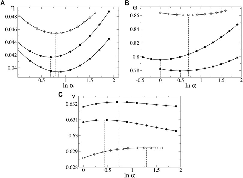
FIGURE 1. Critical exponents η (A), ω (B), and ν (C) vs. ln α provided by the approximate RG flow equations (Sec. 6) of the original BMW scheme (squares), the modified BMW scheme (solid circles), and the scheme of [10] (empty circles), calculated at n = 13, n′ = 10 in (73)–(74). The values obtained using the principle of minimal sensitivity correspond to the extremum points, indicated by the vertical dashed lines.

These PMS values are collected in Table 1. The values in the third row are taken from [36], where the indicated error bars have been estimated based on a detailed analysis of the convergence in (73)–(74). We set the error bars in the first two rows in Table 1 based on a comparative analysis. We performed calculations at n = 10, n′ = 7 and found that the deviations in the critical exponents relative to those for n = 13, n′ = 10 strongly correlate in all three schemes considered and are comparable in magnitude with the corresponding error bars in row 3. For η and ν, these deviations in the BMW schemes are slightly (by 18% for ν and even less for η) larger than those in the scheme of [10]. For ω, they are at least by 38% smaller. In absence of a more detailed convergence test, we rounded up the expected error bars in rows 1–2.

TABLE 1

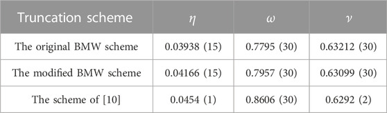
TABLE 1. Values of the critical exponents η, ω, and ν, extracted from approximate RG flow equations (Sec. 6) of three schemes, using the principle of minimal sensitivity to find the optimal parameter α for each of the exponents, as shown in Figure 1.

The critical exponents obtained here for the original BMW scheme coincide with those reported in [17], i.e., η ≈ 0.039, ν ≈ 0.632, and ω ≈ 0.78. The estimates in Table 1 can be compared with those of the conformal field theory (CFT), i. e., η = 0.0362978(20), ν = 0.6299709 [38], and ω = 0.82951(61) [39], which are claimed to be very accurate. This comparison shows that the considered truncated RG equations give rather accurate values of ν, but the values of η are less accurate and somewhat overestimated.

Concerning ω, there are still some doubts about the acceptable value. Probably, the CFT value ω_CFT = 0.82951 (61) is just the acceptable one. However, as discussed in [40], some numerical estimates, including the Monte Carlo renormalization group (MCRG) values ω ≈ 0.7 [42], ω = 0.75 (5) [42], the MCRG estimate from the reanalyzed data of [41] ω = 0.741 (21) [40], and the large mass expansion result ω ≈ 0.8002 [43] tend to give smaller ω values. Seeking for a compromise between these estimations, we set 0.76 as the lower bound for ω in our formal analysis. This choice is partly motivated by the fact that even smaller ω values would poorly fit in this analysis, where the refined estimates are expected to be at least slightly better than those of the LPA.

Thus, we consider ω = ω_CFT as one option, allowing also a theoretical possibility that ω is smaller than ω_CFT, but not smaller than 0.76. In this case, the actual RG estimates of η, ν, and ω in Table 1 are closer to the exact values than the corresponding PMS estimates of LPA, i. e., η_LPA = 0, ν_LPA = 0.650601 (10), and ω_LPA = 0.654115 (30) [36] for the cut-off function (62). It can be seen from the values of the parameter

${\zeta }_{\lambda }=\frac{\lambda -{\lambda }_{ex}}{\lambda -{\lambda }_{\text{LPA}}},(76)$

where λ = η, ν, ω is the actual RG estimate of the critical exponent, λ_ex is its exact value, and λ_LPA is its LPA value. The parameters ζ_λ, calculated from the PMS values of λ and λ_LPA, are collected in Table 2. We evaluated ζ_ω at ω_ex = ω_CFT, ω_ex = 0.8, and ω_ex = 0.76 in (76) to see how this parameter changes if the exact ω value is 0.76 ≤ ω ≤ ω_CFT. It should be noted that ζ_λ > 1/2 would mean that the estimate of λ in Table 1 is worse than that of the LPA. It would be true for λ = ω in the scheme of [10] if ω_ex ≤ 0.757.

TABLE 2

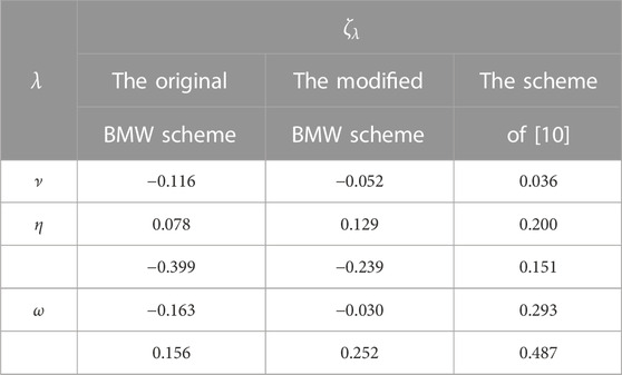
TABLE 2. Parameters ζ_λ with λ = η, ν, ω, calculated from the PMS values of the critical exponents (Table 1) of three truncation schemes. The last three rows contain ζ_ω values for ω_ex = ω_CFT (top), ω_ex = 0.8 (middle), and ω_ex = 0.76 (bottom) in (76).

We further used these parameters for a rough estimation of possible error bars for the subleading correction-to-scaling exponent ω₂ in Sec. 7.3, assuming that $|{\zeta }_{{\omega }_2}|$ does not essentially exceed the largest values of |ζ_λ| for λ = η, ν, ω.

7.3 Estimation of the critical exponent ω₂

The developed techniques allow us to extract from the RG flow not only the leading correction-to-scaling exponent ω but also the subleading one ω₂. To the best of our knowledge, it has not yet been obtained from the Wetterich equation beyond the LPA, where ω₂ ≈ 3.18 has been reported in [15] for the actually considered scalar 3D model.

The RG flow is described by the state vector X depending on t, where X includes all the independent variables contained in the RG flow equations. In particular, considering our semi-analytic approximations, the components of X are the coefficients u_m,k in (73) and the functions f_m,k(y) in (74). The RG flow equations have the form

${\partial }_{t}X=F\left(X,t\right),(77)$

where the explicit t dependence of F (X, t) shows up only in the upper cut-off and is irrelevant in vicinity of the fixed point X = X*. A standard method is to linearize X = X* + δX with respect to an infinitesimal deviation δX from the fixed point. It leads to the solution of the linearized RG, which has the form

$\delta X=C_1{X}_1{e}^{\omega t}+C_2{X}_2{e}^{{\omega }_{2}t}+\mathcal{O}\left(e^{{\omega }_{3}t}\right)(78)$

on the critical surface at large −t values (t < 0), where ω is the leading correction-to-scaling exponent, ω₂ > ω is the subleading correction-to-scaling exponent, ω₃ > ω₂ is the next exponent in this hierarchy of the eigenvalues, and X_i is the eigenvector corresponding to ω_i (where ω₁ ≡ ω). For a unique representation, the eigenvectors are normalized appropriately. The constants C_i depend on the initial conditions.

Our basic idea is to find such initial conditions, at which C₁ = 0. In this case, $\delta X\propto e^{{\omega }_{2}t}=k^{{\omega }_2}$ holds in the linearized RG at t → −∞. Obviously, it holds also beyond the linearized RG since the non-linear corrections are those proportional to ${\left(C_1{e}^{\omega t}\right)}^2$, ${\left(C_1{e}^{\omega t}\right)}^3$, $C_1{C}_2{e}^{(\omega +{\omega }_2)t}$, etc., which are formally contained in $\mathcal{O}\left({(\delta X)}^2\right)$. It means that all terms containing the exponent ω vanish at C₁ = 0. It allows us to extract numerically the exponent ω₂ from the RG flow at C₁ = 0 just as we extracted ω at C₁ ≠ 0.

A direct numerical extraction of ω₂ from the RG flow at C₁ ≠ 0 is difficult since δX contains a full set of correction terms in this case, including all ∝ k^nω terms with integer n ≥ 1. The vanishing of all these ∝ k^nω terms at C₁ = 0 is a great advantage. We strictly verified numerically that these terms really vanish at C₁ = 0. Namely, we have always obtained by our method such ω₂ value, which is not just an integer multiple of ω, despite the fact that nω < ω₂ holds for some n > 1.

We integrated the RG flow with a certain initial condition at k = k₀, where k₀ = Λ = 1, choosing $f_{m,k_0}={\delta }_{m,0}$, $u_{3,k_0}=1$, and $u_{m,k_0}=0$ for m > 3. We set $u_{2,k_0}=0.2$, iteratively adjusting $u_{1,k_0}$ to the critical surface and determining the critical exponents η and ω, as described in Sec. 7.2. For the estimation of ω₂, additional calculations were performed at different values of $u_{2,k_0}$ (adjusting $u_{1,k_0}$ for each of them to fit the critical surface) and finding such $u_{2,k_0}$ value $u_{2,k_0}=u_2^{+}$, at which the condition C₁ = 0 is satisfied. At this condition, amplitude a of the leading scaling behavior $u_{1,k}-u_1^{*}=a{k}^{\omega }$ at k → 0 (where $u_1^{*}$ is the fixed-point value of u_1,k) vanishes, and the scaling $u_{1,k}-u_1^{*}\propto k^{{\omega }_2}$ is observed on the critical surface at k → 0, in agreement with our previous analysis.

Considering the running exponent ω(k) (calculated just as described in Sec. 7.2) for various $u_{2,k_0}$, we observe that ω(k) tends to a certain value ω₂ > ω at a certain $u_{2,k_0}=u_2^{+}$. As an example, we show this in Figure 2 for the equations of the modified BMW scheme at α = 4.5 with n = 13 and n′ = 10 in (73)–(74). We find from this set of curves that $u_2^{+}\approx 0.6548703$ and ω₂ ≈ 1.962. The truncation error in (73)–(74) was roughly estimated as the modulus of the difference (about 0.015) between the actual result and that one obtained at n = 10, n′ = 7. Taking into account also the uncertainty about 0.002 of the estimation in Figure 2 and rounding up the error bars, we have ω₂ = 1.962 (20) in this example. Such results at selected values of α for all three schemes are collected in Table 3, whereas the plots of ω₂ vs. α at n = 13, n′ = 10 are shown in Figure 3.

FIGURE 2

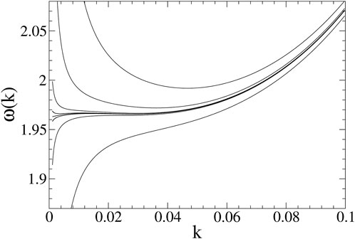
FIGURE 2. Running exponent ω(k) in the modified BMW scheme at α = 4.5. From top to bottom $u_{2,k_0}=0.654$, 0.6547, 0.65485, 0.654867, 0.6548703, 0.654873, 0.6549, and 0.6554. The plot converges to ω₂ ≈ 1.962 at $u_{2,k_0}=u_2^{+}\approx 0.6548703$.

TABLE 3

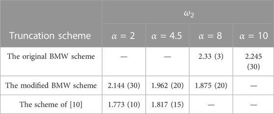
TABLE 3. Subleading correction-to-scaling exponent ω₂, obtained from approximate RG flow equations of three truncation schemes at the given values of parameter α in (62).

FIGURE 3

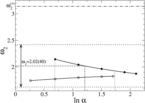
FIGURE 3. ω₂ vs. ln α plots, obtained from approximate RG flow equations of the modified BMW scheme (the upper curve) and the scheme of [10] (the lower curve). The interval α ∈ [1.99, 5.65] of the preferable α values is between the vertical dotted lines. Our final result ω₂ = 2.02 (40), evaluated in the middle of the corresponding ln α interval at α = 3.353 is indicated by the dashed lines, showing the error bars by the horizontal dotted lines and the vertical arrows. The LPA value ${\omega }_2^{\text{LPA}}=3.14(7)$ at α = 3.353 is shown by the horizontal dot–dashed line for comparison.

Because of a poor scaling of ω(k) at $u_{2,k_0}\approx u_2^{+}$, observed in the original BMW scheme at α ≤ 6.7, our ω₂ results for this scheme are limited to α = 8 and α = 10, and the corresponding plot in Figure 3 is not shown. The maximal values of α (8.2 and 5.5), at which the results in the remaining two schemes were obtained, are limited by the problems of finding the solution with C₁ = 0. In addition, the range of α values for the modified BMW scheme is restricted from below by α ≥ 2 because the ω(k) scaling appeared to be relatively poor at a smaller α value (α = 1.3) we considered.

The critical exponents η, ν, and ω are routinely estimated at the PMS values of α. The problem with ω₂ is that no such α values can be identified in Figure 3. Moreover, an extrapolation of the plots in Figure 3 suggests that the extremum points, which could be identified with these PMS values, probably, are located at very large α values of about 20 or even $>20$. The choice of such α values as optimal ones seems to be doubtful since the overall accuracy of the solution is relatively low at α ∼ 20, i. e., η, ν, and ω deviate remarkably from the optimally estimated values.

The estimation can be performed at reasonable values of α, chosen according to some extra criteria. In particular, ω₂ is determined from the RG flow on the critical subsurface, where C₁ = 0 holds; therefore, it makes sense to consider such α values, which allow describing this flow as far as possible accurately. The critical exponents η and ω₂ are relevant for this flow; therefore, we are looking for such α values, which are acceptable or preferable for the estimation of both these exponents simultaneously.

We focus mainly on the estimation of ω₂ from the equations of the modified BMW scheme. This method is advantageous from the point of view that it appears to be much more accurate than the LPA if ω = ω_CFT, as well as if ω has a significantly smaller value within [0.76, ω_CFT]. It is evident from the coefficients ζ_λ in Table 2. We argue that preferable values of α for the estimation of ω₂ from these equations are $\alpha \in [{\alpha }_{\mathit{opt}}^{\eta },5.65]$, where ${\alpha }_{\mathit{opt}}^{\eta }=1.99$ is the optimal α value for the estimation of η. Indeed, both η and ω₂ become more sensitive with respect to the variation of α if α is decreased below ${\alpha }_{\mathit{opt}}^{\eta }$. Therefore, we choose α > 1.99. On the other hand, the deviation from the exact η value monotonously increases with α for $\alpha >{\alpha }_{\mathit{opt}}^{\eta }$ and, at α = 5.65, becomes twice as large as at ${\alpha }_{\mathit{opt}}^{\eta }$. Therefore, we consider α ∈ [1.99, 5.65] as preferable values of α, corresponding to the interval ln α ∈ [0.688, 1.732] between the vertical dotted lines in Figure 3. We choose ln α = 1.21 as an intuitively well-acceptable or nearly optimal ln α value in the middle of this interval. It gives ω₂ = 2.017 (20), as shown in Figure 3 by the dashed lines. The error bars of ω₂ = 2.017 (20) include only the uncertainty of this estimation at ln α = 1.21 or α = 3.353.

The estimation of the total error bars, including the systematic deviation from the exact value due to the closing approximation used in the modified BMW truncation scheme, is based on the assumption that, at appropriate α values (including α = 3.353), $|{\zeta }_{{\omega }_2}|$ does not essentially exceed the largest value 0.252 of |ζ_λ| for λ = η, ν, ω in this scheme, see Table 2. We have set somewhat larger maximal value 0.3 for $|{\zeta }_{{\omega }_2}|$ to increase the confidence level of our estimation. Thus, we evaluated the truncation error bars as $0.3\left|{\omega }_2^{\text{LPA}}-{\omega }_2\right|$, where ${\omega }_2^{\text{LPA}}$ is the LPA value of ω₂ at α = 3.353 and ω₂ = 2.017 (20) is our actual estimate at this α. We obtained ${\omega }_2^{\text{LPA}}=3.14(7)$ at α = 3.353 by our techniques, setting n′ = 0 in (74) and considering n ≤ 13 in (73). This LPA value is close to ${\omega }_2^{\text{LPA}}\approx 3.18$ reported in [15]. Taking into account all error estimates in our calculations, our final result is

${\omega }_2=2.02\left(40\right)(79)$

for the scalar model in three dimensions, which belongs to the 3D Ising universality class. Although the error bars in (79) are not rigorous, no much larger discrepancy with the exact value is expected according to the arguments provided. These arguments basically rely on the assumption that the convergence of ω₂ values, estimated at the truncation orders s = 0, 2, 3, 4, etc., in the modified BMW scheme, would not be essentially slower than the convergence for all other exponents (η, ν, and ω) considered here. Since the actual results include only the cases s = 0 and s = 2, no strict validation of this assumption is possible at the moment; therefore, the error bars in (79) are preliminary. From this point of view, one could allow even larger error bars, but the current information is insufficient to state how much larger. It can be clarified by extended calculations at higher orders.

The error bars of this estimation and the LPA value are shown in Figure 3 for an analysis and comparison. The results extracted from the equations of [10] support (79) since the corresponding lower curve in Figure 3 well fits within these error bars. This estimate agrees also with the RG value ω₂ = 1.67 (11) obtained earlier in [37] from the approximated Polchinski RG equation within the derivative expansion at the $O\left({\partial }^2\right)$ order. The relatively small (as compared to ours) error bars stated for this value presumably reflect only the uncertainty of the estimation from this approximate equation.

8 Summary and outlook

In this section, we give a brief summary of the obtained results, as well as discuss some possible further applications and developments.

In the current paper, we reported our new developments in the BMW truncation scheme for the Wetterich non-perturbative RG equation. We derived explicit RG flow equations for the scalar model at the arbitrary order of truncation, proposing also new closing approximations for the hierarchy of equations for the n-point functions in the BMW scheme (Sec. 4). A surprising similarity between the original and the modified equations of the BMW scheme at s = 2 order of truncation and those recently reported in [10] was shown (Secs. 5–6). As an example, calculations of the critical exponents for the 3D scalar model were performed, solving these equations by the method of semi-analytic approximations recently proposed in [36] (Sec. 7).

Particularly, the subleading correction-to-scaling exponent ω₂ has been evaluated from the Wetterich equation beyond the LPA. Our estimate ω₂ = 2.02 (40) is significantly smaller than the LPA value 3.18 reported in [15] and compares well with the value ω₂ = 1.67 (11), obtained in [37] from the Polchinski equation at the $O\left({\partial }^2\right)$ order of DE. The error bars of our estimate ω₂ = 2.02 (40) are relatively large because they include the expected truncation error due to the closing approximation in the BMW scheme.

The calculations of ω₂ demonstrate the usefulness of our new developments. In particular, just the modified equations of the BMW scheme and those derived in [10] appeared to be practically most useful for these calculations, allowing obtaining the results at reasonable values of the optimization parameter α.

The estimation of the critical exponent ω₂ is crucial for testing the consistency between the RG exponents and those of the CFT. While the RG critical exponents η, ν, and ω appear to be reasonably close to the corresponding CFT values (see Sec. 7.2), there is clearly a problem with ω₂. As already pointed out in Sec. 1, the known estimation in [37] gives a much smaller ω₂ (i. e., ω₂ = 1.67 (11)) than the CFT value 3.8956 (43) [39]. Our current estimation ω₂ = 2.02 (40) allows for significantly larger than 1.67 values; however, these are still very small to speak about a consistency with CFT. In fact, the current estimations urge us to think that the RG exponent ω₂, probably, is unrelated to the conformal symmetry since the RG values appear to be incompatibly smaller than 3.8956 (43).

The proposed scheme has the potential for various applications in calculations at higher than s = 2 orders. In particular, it would help in a further clarification of the question about the relation between the RG exponents and the CFT exponents. Development of improved solution techniques would be quite important for such calculations. Following [44,45], an interesting option is to use the expansion in Chebyshev polynomials for semi-analytic approximations. It could be an advantageous method owing to the guaranteed fast convergence properties of such expansions [45]. These can be used as an alternative to the expansions in powers of z in (73)–(74). One can also think about appropriate semi-analytic approximations for the momentum dependence of the n-point functions to make the calculations at higher than s = 2 orders more feasible.

Apart from very extensive and systematic applications of the non-perturbative RG approach to equilibrium statistical physics, it has also been applied to the out-of-equilibrium systems and critical dynamics [32–34]. The employed truncation schemes include the LPA and its refined modification [34]. There is still room for potential applications of other truncation schemes, including the currently introduced modified BMW scheme, which could be adjusted to this problem. It would be a quite interesting application, eventually, allowing obtaining refined RG estimates for the dynamical exponent z. Indeed, the actual estimates of this exponent are not very accurate, and there is a continued discussion of z values obtained from Monte Carlo simulations, experiments, and RG equations [34, 46].

Data availability statement

The raw data supporting the conclusion of this article will be made available by the authors, without undue reservation.

Author contributions

All authors listed made a substantial, direct, and intellectual contribution to the work and approved it for publication.

Acknowledgments

The authors acknowledge the Latvian Grid Infrastructure and High Performance Computing Centre of Riga Technical University for providing resources. JK acknowledges the support from the Science Support Fund of Riga Technical University. RM acknowledges the support from the NSERC and CRC programs.

Conflict of interest

The authors declare that the research was conducted in the absence of any commercial or financial relationships that could be construed as a potential conflict of interest.

Publisher’s note

All claims expressed in this article are solely those of the authors and do not necessarily represent those of their affiliated organizations, or those of the publisher, the editors, and the reviewers. Any product that may be evaluated in this article, or claim that may be made by its manufacturer, is not guaranteed or endorsed by the publisher.

Supplementary material

The Supplementary Material for this article can be found online at: https://www.frontiersin.org/articles/10.3389/fphy.2023.1182056/full#supplementary-material

References

1. Amit DJ. Field theory, the renormalization group, and critical phenomena. Singapore: World Scientific (1984).

Google Scholar

2. Sornette D. Critical phenomena in natural sciences. Berlin, Germany: Springer (2000).

Google Scholar

3. Shang–Keng Ma. Modern theory of critical phenomena. New York, NY, USA: W.A. Benjamin, Inc. (1976).

Google Scholar

4. Zinn–Justin J. Quantum field theory and critical phenomena. Oxford, England: Clarendon Press (1996).

Google Scholar

5. Kleinert H, Schulte–Frohlinde V. Critical properties of ϕ⁴ theories. Singapore: World Scientific (2001).

Google Scholar

6. Wetterich C. Exact evolution equation for the effective potential. Phys Lett B (1993) 301:90. doi:10.1016/0370-2693(93)90726-X

CrossRef Full Text | Google Scholar

7. Polchinski J. Renormalization and effective Lagrangians. Nucl Phys B (1984) 231:269. doi:10.1016/0550-3213(84)90287-6

CrossRef Full Text | Google Scholar

8. Bagnuls C, Bervillier C. Exact renormalization group equations. An introductory review. Phys Rep (2001) 348:91. doi:10.1016/S0370-1573%2800%2900137-X

CrossRef Full Text | Google Scholar

9. Berges J, Tetradis N, Wetterich C. Non-perturbative renormalization flow in quantum field theory and statistical physics. Phys Rep (2002) 363:223. doi:10.1016/S0370-1573%2801%2900098-9

CrossRef Full Text | Google Scholar

10. Kaupužs J, Melnik RVN. A new method of solution of the Wetterich equation and its applications. J Phys A: Math Theor (2020) 53:415002. doi:10.1088/1751-8121/abac96

CrossRef Full Text | Google Scholar

11. Balog I, Chate H, Delamotte B, Marohnic M, Wschebor N. Convergence of nonperturbative approximations to the renormalization group. Phys Rev Lett (2019) 123:240604. doi:10.1103/PhysRevLett.123.240604

PubMed Abstract | CrossRef Full Text | Google Scholar

12. Papenbrock T, Wetterich C. Two-loop results from improved one loop computations. Z Phys C (1995) 65:519. doi:10.1007/BF01556140

CrossRef Full Text | Google Scholar

13. Litim D. Optimized renormalization group flows. Phys Rev D (2001) 64:105007. doi:10.1103/PhysRevD.64.105007

CrossRef Full Text | Google Scholar

14. Canet L, Delamotte B, Mouhanna D, Vidal J. Optimization of the derivative expansion in the nonperturbative renormalization group. Phys Rev D (2003) 67:065004. doi:10.1103/PhysRevD.67.065004

CrossRef Full Text | Google Scholar

15. Litim DF. Critical exponents from optimised renormalisation group flows. Nucl.Phys B (2002) 631:128. doi:10.1016/S0550-3213(02)00186-4

CrossRef Full Text | Google Scholar

16. Bender CM, Sarkar S. Asymptotic analysis of the local potential approximation to the Wetterich equation. J Phys A: Math Theor (2018) 51:225202. doi:10.1088/1751-8121/aabf63

CrossRef Full Text | Google Scholar

17. Benitez F, Blaizot J-P, Chate H, Delamotte B, Mendez-Galain R, Wschebor N. Non-perturbative renormalization group preserving full-momentum dependence: implementation and quantitative evaluation. Phys Rev E (2012) 85:026707. doi:10.1103/PhysRevE.85.026707

PubMed Abstract | CrossRef Full Text | Google Scholar

18. De Polsi G, Balog I, Tissier M, Wschebor N. Precision calculation of critical exponents in the O(N) universality classes with the nonperturbative renormalization group. Phys Rev E (2020) 101:042113. doi:10.1103/PhysRevE.101.042113

PubMed Abstract | CrossRef Full Text | Google Scholar

19. Berges J, Jungnickel D-U, Wetterich C. Two flavor chiral phase transition from nonperturbative flow equations. Phys Rev D (1999) 59:034010. doi:10.1103/PhysRevD.59.034010

CrossRef Full Text | Google Scholar

20. Schütz F, Kopietz P. Functional renormalization group with vacuum expectation values and spontaneous symmetry breaking. J Phys A: Math Gen (2006) 39:8205. doi:10.1088/0305-4470/39/25/S28

CrossRef Full Text | Google Scholar

21. Benedetti D, Groh K, Machado PF, Saueressig F. The universal RG machine. JHEP (2011) 06:079. doi:10.1007/JHEP06(2011)079

CrossRef Full Text | Google Scholar

22. Demmel M, Saueressig F, Zanusso O. RG flows of Quantum Einstein Gravity on maximally symmetric spaces. JHEP (2014) 06:026. doi:10.1007/JHEP06(2014)026

CrossRef Full Text | Google Scholar

23. Wetterich C, Yamada M. Variable Planck mass from the gauge invariant flow equation. Phys Rev D (2019) 100:066017. doi:10.1103/PhysRevD.100.066017

CrossRef Full Text | Google Scholar

24. Platania AB. Asymptotically safe gravity: from spacetime foliation to cosmology. Berlin, Germany: Springer (2018). p. 29–46.

CrossRef Full Text | Google Scholar

25. Wetterich C. Quantum correlations for the metric. Phys Rev D (2017) 95:123525. doi:10.1103/PhysRevD.95.123525

CrossRef Full Text | Google Scholar

26. Eichhorn A. An asymptotically safe guide to quantum gravity and matter. Front Astron Space Sci (2019) 5:47. doi:10.3389/fspas.2018.00047

CrossRef Full Text | Google Scholar

27. Alwis SP. Exact RG flow equations and quantum gravity. JHEP (2018) 03:118. doi:10.1007/JHEP03(2018)118

CrossRef Full Text | Google Scholar

28. Litim DF, Trott MJ. Asymptotic safety of scalar field theories. Phys Rev D (2018) 98:125006. doi:10.1103/PhysRevD.98.125006

CrossRef Full Text | Google Scholar

29. Bond AD, Litim DF. Price of asymptotic safety. Phys Rev Lett (2019) 122:211601. doi:10.1103/PhysRevLett.122.211601

PubMed Abstract | CrossRef Full Text | Google Scholar

30. Falls KG, Litim DF, Schroder J. Aspects of asymptotic safety for quantum gravity. Phys Rev D (2019) 99:126015. doi:10.1103/PhysRevD.99.126015

CrossRef Full Text | Google Scholar

31. Lahoche V, Samary DO. Progress in solving the nonperturbative renormalization group for tensorial group field theory. Universe (2019) 5:86. doi:10.3390/universe5030086

CrossRef Full Text | Google Scholar

32. Canet L, Chate H. General framework of the non-perturbative renormalization group for non-equilibrium steady states. J Phys A (2007) 40:1937. doi:10.1088/1751-8113/40/9/002

CrossRef Full Text | Google Scholar

33. Canet L, Chate H, Delamotte B. General framework of the non-perturbative renormalization group for non-equilibrium steady states. J Phys A: Math Theor (2011) 44:495001. doi:10.1088/1751-8113/44/49/495001

CrossRef Full Text | Google Scholar

34. Roth JV, Smekal L. Critical dynamics in a real-time formulation of the functional renormalization group (2023). https://arxiv.org/pdf/2303.11817.pdf.

CrossRef Full Text | Google Scholar

35. Dupuis N, Canet L, Eichhorn A, Metzner W, Pawlowski JM, Tissier M, The nonperturbative functional renormalization group and its applications. Phys Rep (2021) 910:1. doi:10.1016/j.physrep.2021.01.001

CrossRef Full Text | Google Scholar

36. Kaupužs J, Melnik RVN. Functional truncations for the solution of the nonperturbative RG equations. J Phys A: Math Theor (2022) 55:465002. doi:10.1088/1751-8121/ac9f8c

CrossRef Full Text | Google Scholar

37. Newman KE, Riedel EK. Critical exponents by the scaling-field method: the isotropic N-vector model in three dimensions. Phys Rev B (1984) 30:6615. doi:10.1103/PhysRevB.30.6615

CrossRef Full Text | Google Scholar

38. Poland D, Simmons-Duffin D. The conformal bootstrap. Nat Phys (2016) 12:535. doi:10.1038/nphys3761

CrossRef Full Text | Google Scholar

39. Reehorst M. Rigorous bounds on irrelevant operators in the 3d Ising model CFT. JHEP (2022) 09:177. doi:10.1007/JHEP09(2022)177

CrossRef Full Text | Google Scholar

40. Kaupužs J, Melnik RVN. Corrections to scaling in the 3D Ising model: A comparison between MC and MCRG results. Int J Mod Phys C (2023):2350079. doi:10.1142/S0129183123500791

CrossRef Full Text | Google Scholar

41. Gupta R, Tamayo P. Critical exponents of the 3D Ising model. Int J Mod Phys C (1996) 7:305–19. doi:10.1142/S0129183196000247

CrossRef Full Text | Google Scholar

42. Ron D, Brandt A, Swendsen RH. Surprising convergence of the Monte Carlo renormalization group for the three-dimensional Ising model. Phys Rev E (2017) 95:053305. doi:10.1103/PhysRevE.95.053305

PubMed Abstract | CrossRef Full Text | Google Scholar

43. Yamada H. Critical exponents from large mass expansion (2014). https://arxiv.org/pdf/1408.4584.pdf.

Google Scholar

44. Borchardt J, Knorr B. Global solutions of functional fixed point equations via pseudospectral methods. Phys Rev D (2015) 91:10. doi:10.1103/PhysRevD.91.105011

CrossRef Full Text | Google Scholar

45. Borchardt J, Knorr B. Solving functional flow equations with pseudospectral methods. Phys Rev D (2016) 94:025027. doi:10.1103/PhysRevD.94.025027

CrossRef Full Text | Google Scholar

46. Zhang W, Barkema GT, Pauja D, Ball RC. Critical dynamical exponent of the two-dimensional scalar ϕ⁴ model with local moves. Phys Rev E (2018) 98:062128. doi:10.1103/PhysRevE.98.062128

CrossRef Full Text | Google Scholar