Automatic Generation of Randomized Trial Sequences for Priming Experiments

In most psychological experiments, a randomized presentation of successive displays is crucial for the validity of the results. For some paradigms, this is not a trivial issue because trials are interdependent, e.g., priming paradigms. We present a software that automatically generates optimized trial sequences for (negative-) priming experiments. Our implementation is based on an optimization heuristic known as genetic algorithms that allows for an intuitive interpretation due to its similarity to natural evolution. The program features a graphical user interface that allows the user to generate trial sequences and to interactively improve them. The software is based on freely available software and is released under the GNU General Public License.

1 Introduction

In almost all psychological research that applies an experimental strategy, randomization of stimuli, participants and/or experimental conditions is essential for the validity of the obtained results. Many paradigms are simple enough that an on-line randomization can be applied, i.e., the experimental software can determine the stimuli to be shown by itself (e.g., by randomly choosing a stimulus from a given set). Some experimental setups, however, feature complex inter-trial dependencies such that proper randomization is more difficult. Consider for example negative priming (NP) experiments (e.g., Tipper, 1985). In these paradigms, the experimental condition of a trial depends not only on the stimuli presented in the trial (probe) but also on the preceding trial (prime). This dependency between trial i and trial i − 1 makes proper randomization difficult (because the condition in trial i + 1, in turn, depends on the stimuli in trial i). This paper presents a software that was designed to generate randomized stimulus-sequences for (negative-) priming experiments based on a heuristic optimization method known as genetic algorithms (GAs).

For illustration, we present a standard NP study (Schrobsdorff et al., 2007) which we will use as a reference throughout the manuscript to clarify the exposition of our methodology. In their study, Schrobsdorff et al. (2007) presented pictograms of everyday objects (ball, book, bench, boat, bed) in two different colors and required their subjects to voice the label of the green stimulus while ignoring the red stimulus (see Figure 2). Repetition priming and NP are realized by repeating one or both (partial vs. full repetition) of the objects from prime to probe either in the same (positive priming) or reversed colors (NP). The basic result is that reaction times and error rates are reduced for identical repetitions while they are increased for distractor-to-target repetitions (in relation to a control condition where no stimuli are repeated).

Randomization of stimulus presentation is of particular importance in such priming experiments because it is known that the emergence of priming effects depends on the mix of priming conditions in the realized trial-sequence. The NP effect, for example, is influenced by the proportion of attended and ignored repetition trials, respectively (Frings and Wentura, 2008). NP also depends on many subtle sequence-related factors such as number of stimuli (Kramer and Strayer, 2001) and stimulus-repetitions (for a review see Fox, 1995). It is therefore essential for the validity of the study to (1) present an exact proportion of stimuli/conditions as specified by the experimenter and (2) to randomize everything else properly.

Negative priming experiments are sometimes conducted using a “blocked” trial-presentation scheme that presents prime and probe as a single trial (usually, prime-probe episodes are distinguished by a longer interval between the trials than between prime and probe, e.g., Milliken et al., 1998; Grison and Strayer, 2001; Rothermund et al., 2005; Frings and Wentura, 2006). This approach has the advantage that experimental conditions are easily randomized because the prime-probe pairs are independent of one another. However, there are also problems with this approach: First, possible influences of the display that precedes prime-onset (the probe of the preceding trial) are disregarded and explicitly removed from the analysis. Since these probe-prime transitions are not controlled, overrepresentations of some probe-prime combinations may occur. Since it is known that the proportions of repeated stimuli may influence the overall pattern of results (e.g., Frings and Wentura, 2008), this can be problematic for the interpretation of the results unless probe-prime transitions are explicitly analyzed and reported. There is also evidence for long-term priming effects (e.g., Lowe, 1998; Grison et al., 2005) as well as for the emergence of second-order priming effects (e.g., mediated priming; Livesay and Burgess, 1998) which further question the practical applicability of blocked trial-presentation. Last but not least, the experimental efficiency is reduced by half of what could be achieved by continuous presentation. As a consequence, the time required for the experimental session increases, potentially causing mental fatigue which is associated with loss of cognitive control (Lorist et al., 2005) which in turn appears to be a prerequisite for NP to occur (de Fockert et al., 2010).

Continuous presentation schemes in which trial i is the probe for trial i − 1 and the prime for trial i + 1 (e.g., Kramer and Strayer, 2001; Titz et al., 2008; Behrendt et al., 2010) circumvent these problems but also make randomization much harder. This is due to the fact that the trials are not independent anymore: Changing the stimuli in display i changes the experimental condition of trial i and trial i + 1. This dependency makes a randomized presentation of stimuli over the complete sequence very difficult when factors such as the number of presented trials for each priming condition are to be balanced across the experiment. A pseudo-randomized trial-presentation is often used where the stimuli are selected based on a list that fulfills the desired properties. Generating such lists is not trivial because of the cross-trial dependencies. In addition, regarding trial-sequence generation as an optimization problem, there may not exist a perfect solution such that the “optimal” sequence will necessarily violate some of the experimental constraints.

Furthermore, care must be taken that the sequences do not induce the use of strategies by the participants. For example, in NP tasks, subjects could use the prime distractor to predict the probe target (May et al., 1995) if they were aware of the experimental manipulation. The presentation of “random” (in the sense of unpredictable) trial sequences is therefore necessary. The literature on implicit sequence learning suggests that participants are able to exploit regularity in trial sequences for responding (Stadler, 1992; Stadler and Neely, 1997; Boyer et al., 2005) even if this regularity is quite subtle as, e.g., when the sequence is generated by an abstract grammar (Visser et al., 2009). To ensure “unpredictability,” many experimentalists control the presented trial-sequence in a way that some structural criteria are fulfilled. For example, it is desirable that the trials do not come in predictable patterns (e.g., multiple consecutive instances of the same experimental condition) and that stimuli appear an equal number of times. This is a tricky aspect, though: In an information-theoretic sense, any additional constraint (e.g., avoiding consecutive trials of the same experimental condition) on stimulus-sequences will reduce the entropy (the theoretical unpredictability) of the process that generated them (for an introduction to information theory, see Cover and Thomas, 2006). However, humans are more affected by local regularities and it is therefore desirable to avoid local structure in the sequences (see literature on implicit sequence learning, e.g., Stadler, 1992). The criteria applied in the design of the trial sequences are only loosely defined because it is unclear what regularities have to be avoided in order to ensure unpredictability. This poses a difficulty to computer-aided trial-sequence generation as all constraints must be formally specified. In addition, any automated optimization technique must allow for deviations from the optimum and be flexible enough to adapt to different experimental needs.

In this paper, we present a computer program that makes use of a global optimization heuristic known as genetic algorithms (GAs) (Goldberg, 1989) to generate and optimize stimulus-sequences for priming experiments. As the name suggests, GAs are inspired by natural evolution and the parameters have therefore a natural equivalent in evolutionary biology. This fact allows for an intuitive understanding of how parameter changes will affect the results which is very useful when working with the optimization algorithm. Our program allows to generate trial sequences for a variety of priming tasks. All priming paradigms that include two dimensions on which stimuli are distinguishable are supported. This includes in particular naming and categorization tasks in semantic or identity priming paradigms but also other tasks, such as priming in visual search (Kristjánsson and Driver, 2008).

In the following, we will shortly outline the theory of GAs. Furthermore, we will present the program and explain how it can be used to generate trial sequences for specific experiments. Finally, we present examples of results acquired using the program, compare it to an on-line randomization approach and discuss potential extensions.

2 Materials and Methods

2.1 Genetic Algorithms

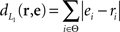
Genetic algorithms are search heuristics that can be used to approximate a globally optimal solution to a problem. GAs have been successfully applied to many real-life problems in fields as different as economics, biology, and computer science (Goldberg, 1989). The approach is inspired by biological evolution: It mimics concepts like inheritance, mutation, natural selection, and recombination (Beasley et al., 1993a,b). Basically, the algorithm generates random solutions to the problem and improves them by means of evolutionary strategies. The operation of the algorithm therefore requires a way to generate solutions from the space of all possible solutions 𝒮 to the optimization problem and a fitness function ℱ:𝒮 → [0,1] that assigns a real number (fitness value) to each member of 𝒮.

The performance of the GA depends more on the choice of an efficient encoding scheme and the fitness function than on the settings of other more peripheral parameters. Therefore, a first problem is to find a suitable representation of valid solutions. In allusion to the biological equivalent, such a representation is called a genome, g ∈ 𝒮. The classical version of the GA requires a binary coding of the input (Goldberg, 1989): For example, if any solution can be coded as a sequence of arbitrary integer numbers, these can be represented as binary strings following the standard decimal to binary conversion. However, it is often beneficial to use a representation that is specifically tailored to the search-space and does not allow “invalid” solutions to be coded. We therefore implement a genome designed to encode exactly the valid stimulus-sequences but not more (see Section 2.2.2).

The second and most important step to apply a GA to an optimization problem is to design the fitness or objective function ℱ. This function takes an instance of the set of all possible solutions and evaluates it in terms of how well it solves the problem, i.e., it assigns a score, the “fitness,” to it. The design of this function is crucial for the performance of the algorithm as it is the only means for the algorithm to determine the efficiency of a generated solution, thereby governing the result of the optimization completely.

There are several variants of GAs but the general behavior is as follows: A random initial population 𝒫₀ = {g₁,…,gN} of N possible solutions is generated and a fitness value is calculated for each genome. Then, a reproductive cycle is started in which two instances from 𝒫₀ are sampled according to their fitness which are used to generate two offspring (i.e., members of the next population 𝒫₁) by recombination. With probability p_mut, each genome from a population undergoes a mutation (i.e., one bit of the genome is flipped, see Figure 1B). There are several possible schemes for recombination (Beasley et al., 1993a), the most classical being cross-over where parent genomes are split at a random location and recombined with probability p_cross (see Figure 1A). The natural selection is represented by the fitness-biased selection of genomes for recombination from the parent population. This step is repeated until the children-population is again of size N. The parent population is then dropped and the whole procedure iterated with the new population as parent population, thereby generating a sequence of populations 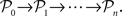The iterations end when either a maximum number of generations has been reached or the mean fitness of the population saturates (i.e., the algorithm converges).

FIGURE 1

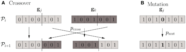
Figure 1. Cross-over and mutation. (A) Two individual genomes are chosen from the parent population 𝒫_i and recombined using the cross-over technique to yield two members of the children-population 𝒫_{i + 1}. The splitting point is chosen randomly. (B) When going from population 𝒫_i to 𝒫_{i + 1}, each bit is flipped with probability p_mut, mimicking the effect of mutation in natural evolution.

Maybe an image is helpful to illustrate these rather technical explanations: Picture a population of rabbits living on a desolate island. The island holds enough resources to support only N individual rabbits (this is the population size parameter). There are some dangers on the island (high waves, predator animals) such that evolutionary pressure (the fitness function) encourages the mating and reproduction of fitter individuals (the reproductive cycle). During reproduction, the rabbit’s genomes are recombined (cross-over) and are subject to random mutations such that child rabbits may differ considerably from their parents. Because the island can hold only N rabbits, for each child rabbit, one of the adult ones must perish. No child can perish before all adults are gone and after all adult rabbits have died, the new population begins reproducing. This corresponds to one iteration of the GA and continues until a specified number of generations have lived on the island. With such a picture in mind, it is easy to attach meaning to the parameters of the optimization algorithm and to predict how a parameter change might influence the results.

2.2 Application to Trial-sequence Generation

In order to apply GAs to the problem of trial-sequence generation, a coding scheme must be devised allowing to encode trial sequences in a way that the genetic operators cross-over and mutation can be applied such that they yield valid solutions. Furthermore, a fitness function needs to be specified that encodes the experimental requirements and that makes the sometimes implicitly given requirements and assumptions explicit.

2.2.1 Scope of the approach

We formalize the experimental setup as follows: There are two different “types” of stimuli (i.e., target and distractor) and a number of stimulus “identities” (e.g., specific words or pictures) which are indexed by integer numbers ranging from 1 to n_stim. Experimental conditions are defined by which stimuli repeat from one trial to the next. All possible repetitions of one or both stimuli are supported as shown in Table 1.

TABLE 1

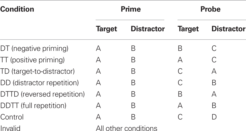
Table 1. Stimulus-repetition conditions supported by our framework.

In our reference study (Schrobsdorff et al., 2007), the set of stimuli comprises the n_stim = 5 objects ball, book, bench, boat, and bed. Each of these stimuli can be the target (when it is presented in green) or the distractor (red). The study implemented priming conditions with both partial (DT, TT) and full repetitions (DTTD, DDTT), see Figure 2. The software was designed with such identity NP experiments in mind but is also applicable to other priming paradigms. In fact, all priming paradigms that include two dimensions on which stimuli are distinguishable are supported. This includes in particular naming and categorization tasks in semantic or identity priming paradigms but also other tasks, such as priming in visual search (Kristjánsson and Driver, 2008).

FIGURE 2

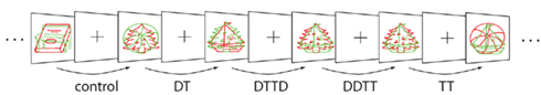
Figure 2. Stimuli and conditions used in a reference negative priming study (Schrobsdorff et al., 2007, see Table 1 for the abbreviations).

It is also possible to use the software for generating trial sequences for semantic or affective priming tasks, even though a bit of additional work is required. Consider for example the study by Damian (2000) in which priming between same-category stimuli (vehicles, tools, animals, furniture, and clothing) was investigated. Priming was investigated by considering, e.g., whether subsequent presentation of two different tools or vehicles primed each other. In this case the categories, not the actual instances, would correspond to stimuli in our software. The mapping from category to specific object would have to occur after the sequence has been generated and is out of the scope of the software. However, this is relatively straight-forward using a spreadsheet software to replace category-labels with instances (though care must be taken to randomize the number of occurrences of each stimulus as well). We will discuss potential extensions of our software in the general discussion.

2.2.2 Coding and genetic operators

Currently only sequences for two distinct types of stimuli (“targets” and “distractors”) can be realized. A trial-sequence “genome” g = (t,d), thus consists of two sequences (t_i,d_i) ∈ {1,…,n_stim} × {1,…,n_stim} with i ∈ {1,…,n_trials} each of which codes for one of the n_stim possible stimuli¹. Thus, the genome g is a sequence of numbers indicating which stimulus is presented as target and distractor in each trial and 𝒮 is the set of all possible trial sequences. In our reference study, a typical genome looks like that in Table 2. We define the genetic operators cross-over 𝒞 : 𝒮 × 𝒮 → 𝒮 (defining sexual reproduction by combining two genomes) and mutation 𝓜 : 𝒮 → 𝒮 (defining a mutational change of the genome) such that they must produce valid solutions. The cross-over operator randomly determines a trial at which to split the genome and concatenates the parent genomes such that the child is identical to the “father” up to the split point and identical to the “mother” thereafter. The mutation operator simply replaces each stimulus (either in t or in d) independently with a random element from {1,…,n_stim} with probability p_mut (i.e., the probability that there is at least one mutation in a genome is 2n_trialsp_mut and is typically very small).

TABLE 2

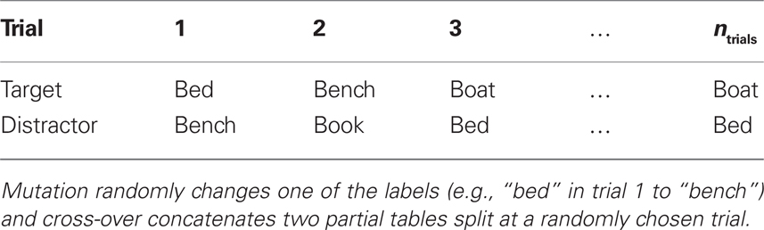
Table 2. Typical genome for the reference study (Schrobsdorff et al., 2007).

2.2.3 Fitness function

We chose a fitness function ℱ:𝒮 → [0,1] for trial-sequence generation that evaluates a solution in terms of a weighted sum of a number of n_crit separate criteria C_i:𝒮 → [0,1] that are rescaled according to a power-law with exponent k

The weights ω_i ∈ [0,1] are restricted to sum to 1 and can be adjusted by the user to emphasize the importance of some of the criteria. The scaling exponent k can be chosen to give more emphasis to low scores when the overall convergence behavior is not satisfactory (i.e., the algorithm converges at low fitness values, e.g., 0.8).

The following n_crit = 5 criteria were implemented in our software:

(i) only desired priming conditions are realized (e.g., in the reference study, only control, DT, TD, DTTD, and DDTT trials are presented),

(ii) priming conditions appear a desired number of times [e.g., each condition was to appear 80 times in Schrobsdorff et al. (2007)study],

(iii) only three consecutive trials of the same condition are allowed,

(iv) all objects appear as target an equal number of times (e.g., there have to be as many target “benches” as target “books”),

(v) all objects appear as distractor an equal number of times (e.g., there have to be as many distractor “benches” as distractor “books”).

The choice of these criteria reflects an attempt to find the minimal number of criteria such that the software produces sequences that do not show any obvious structure. Additional criteria (e.g., the distribution of objects per priming condition) are usually fulfilled when a large number of trials is generated. The implementation of more or alternative criteria is straight-forward, but requires programming skills because the source-code of the application needs to be adapted.

Only desired priming conditions. This criterion is implemented as the number of trials of desired experimental conditions divided by the number of all trials,

Desired distribution of priming conditions. The user can specify a desired distribution r_i giving the relative number of times each of the priming conditions i ∈ Θ: = {control, DT, TT, TD, DD, DDTT, DTTD} should occur in the generated sequence. To calculate this criterion, we have to compare the empirical distribution e_i = n_i/n_trials (where n_i is the number of trials of priming condition i, i.e., e_i is the relative frequency of trials of priming condition i) against the desired distribution r_i. The L₁ distance

is a suitable measure, since the maximum of is 2 (if Σ_ie_i = 1 and Σ_ir_i = 1) and the criteria can therefore be calculated to lie within the range [0,1] such that a weighted sum of the criteria can be interpreted. The criterion can then be expressed as

Only three consecutive trials of same condition. All trials that lie in a consecutive sequence of more than three trials of the same condition are counted as n_consecutive. The criterion evaluates to

Uniform distribution of stimuli over target/distractor. These criteria are evaluated similar to the second one by calculating the L₁ distance between a uniform distribution and the empirical distribution. The empirical distribution is the relative frequency each stimulus appears as target/distractor, thus

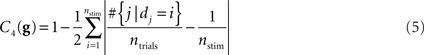
and

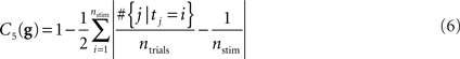
where #S is the number of elements (cardinality) of set S.

After the separate criteria C₁ to C₅ are calculated, they are combined into an overall fitness-score ℱ according to Eq. 1.

2.3 Software Implementation

The program is available as source-code and pre-compiled binaries for a variety of platforms (Microsoft Windows, Mac OS X, Linux 32/64 bit) from the project webpage (Ihrke, 2011) and is released under the GNU General Public License² (Free Software Foundation, 1991). The software comes with a graphical user interface (see Figure 3) allowing to vary all important parameters. Documentation and installation instructions are available from the project webpage and from within the application (“Help”-tab).

FIGURE 3

Figure 3. Screenshot of the “result”-tab. Statistics are located next to a table containing the generated trial-sequence, making it easy to modify and evaluate the sequence.

There are two separate tabs that are designated to set the experimental constraints and the optimization parameters for the GA, respectively. After providing the experimental constraints, the user can hit the “Go” button and the GA will begin the optimization. After the GA has converged, the best sequence found during the optimization is presented in the “Result”-tab along with descriptive statistics. This sequence can be saved as a comma-separated list and, e.g., imported into a spreadsheet program (import via comma-separated values, CSV) or read by the experimental software. On the project’s webpage (Ihrke, 2011), we provide example code for several commonly used presentation environments that read our file-format, thus making the generated sequence accessible to the presentation routine. Furthermore, a plot of the algorithm’s convergence is provided, showing the fitness-score of the worst, average, and best individual over successive populations. This allows the user to directly assess how well the algorithm converged and to judge the quality of the final sequence. Also, the generated sequence can be modified in place and re-evaluated. Finally, a configuration can be saved to file and re-loaded into the application.

2.3.1 Tutorial – suggested workflow

Getting the best result out of the optimization can be tricky when the conditions posed by the experimenter are hard to fulfill. That means, depending on the actual requirements, the optimization problem might be very difficult or the optimal solution might not be good enough because there is no trial-sequence that can come close to satisfying the constraints. Our experience in working with the program resulted in a typical workflow: First, the number of stimuli and the choice of experimental conditions are set along with the length of the trial sequence and the desired distribution of the stimulus-repetition conditions. Then, a first run with the default parameters is executed to check the general level of the solution’s fitness. If the results are unsatisfactory because the sequences do not fulfill the constraints, the GA settings should be manipulated first (i.e., larger population size, more populations) and the resulting increase in performance be evaluated. If the algorithm is observed to converge (when the curve approaches an asymptote) and the performance is still suboptimal, it is necessary to increase the number of trials and/or the number of objects in the sequence since a good solution does not seem to exist. Finally, once a good sequence has been generated, it can be manually tweaked to further increase the fitness. In the following, we give a detailed account of this procedure.

(i) Setting experimental constraints

The first step is obviously to specify the requirements of the planned experiment. The parameters are collected in the “Setup”-tab of the program: Number of stimuli in the experiment, number of trials and the stimulus-repetition conditions along with the desired frequency of the conditions. Depending on the choice of these parameters, the difficulty of the optimization problem is going to vary: It is for example comparatively easy to realize an overrepresentation of control trials because they leave the algorithm the freedom to choose four different stimuli without constraints. In contrast, if many full repetition (DDTT) or reversed repetition (DTTD) trials are desired the constraints may be severe and, in fact, not possible to fulfill completely.

(ii) Running the optimization

It is suggested that an initial run using the default parameter settings is performed. The default parameters have been carefully selected to be successful for a number of requirements. The main parameter is the “number of generations”: It directly determines how many iterations are run and should be the first to be increased. In the next steps the results of the algorithm need to be validated and adjusted to yield optimal results.

(iii) Checking algorithm convergence

The “Convergence”-tab presents a plot of the population scores as a function of population index similar to Figure 4. The user should verify that the score has settled at a high level and does not continue to grow. If the scores have not yet converged, the number of generations should be increased and the algorithm rerun. The default number of generations was set to an intermediate value (5000 generations) in order to provide a fast initial result. The program’s runtime will increase proportionally to the number of generations. If the initial run was fast enough, the number of generations can safely be doubled or tripled (resulting in a run twice or three times as long) to see whether additional value can be gained by longer convergence. Note, that the number of iterations required to solve the problem is dependant on the number of trials in the genome: The longer the trial-sequence, the more iterations have to be run to find a good solution (since the search-space is much larger).

(iv) Check best genome

The “Result”-tab provides an editable table showing the best sequence encountered during optimization along with a graphical summary of the properties of the sequence: There are histograms showing the distribution of the stimuli as target and as distractor and a histogram for the distribution of experimental conditions. The desired distribution is depicted in dark gray for easy orientation (Figure 3). Finally, the partial scores defined in Section 2.2.3 are listed, giving an indication of the quality of the sequence.

(v) In case of good convergence but poor results: Increase degrees of freedom

Occasionally, if experimental parameters are unfortunately selected, the GA may converge at a suboptimal level. In this case, increasing the number of iterations will not solve the problem as the algorithm is stuck in a local maximum. There are a couple of parameters that can be tweaked to provide the algorithm with more flexibility. However, the described steps may also result in a much larger number of necessary iterations and can even prevent the GA from converging at all.

Different steps should be taken, depending on the distribution of the criterion scores:

• One score low, all others high

Sometimes, a good global score can be achieved by choosing a “loser” criterion score that will take on low values while all others can achieve better ones. For example, if a large number of full repetitions (DDTT) are desired, the algorithm could choose to disregard the “only three consecutive same-condition-trials” criterion and produce a large number of consecutive full repetitions. As a remedy, a larger value of k (the power-law-scaling exponent) can be used. This will increase the penalty given to low values of the partial scores. Increasing the weight for the loser-criterion might help as well but can also lead to a different loser being chosen by the algorithm.

• All scores low

When the algorithm converges at a low level for all partial scores, several remedies can be tried: At first the simple GA should be examined (instead of the default steady-state GA). This algorithm is more flexible and convergence will be slower. If the convergence is still good but at a low value, the “elitism” checkbox can be unchecked increasing variability even more. Additionally, larger populations or larger probabilities of mutation and cross-over can help in this situation (also in combination with a steady-state algorithm). The algorithm should be rerun several times to check whether the convergence is reproducible.

(vi) Manual tuning

Finally, the software provides facilities to change and re-evaluate the sequence according to the discussed criteria. The first few best sequences encountered during the run are put into the table in the “Result”-tab (they can be cycled through using the arrow-buttons). It is possible to manipulate items in the sequence and generate a new score on-the-fly which is very convenient for manipulating a close-to-optimal sequence. Such fine-tuning may be desired, when the algorithm included unwanted experimental conditions (which may happen because of the trade-off over the criteria in Eq. 1).

FIGURE 4

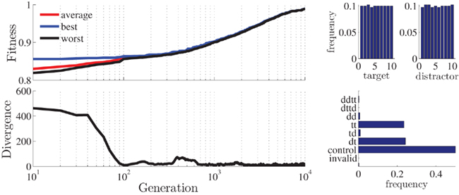
Figure 4. Statistics for the best stimulus-sequence generated with the standard setup. Plotted are the fitness and divergence (average distance between individuals in the population) values as a function of generation (upper and lower left; log-scale) and histograms for target/distractor stimuli (upper right) and stimulus condition (lower right).

Note that it might in general be more practical to generate shorter segments of trial sequences (e.g., one for each experimental block). This is because (i) their generation is easier to control and (ii) they can be combined in randomized order in the experiment without taking care of the trials on the boundary between two blocks. In addition, the final full sequence will satisfy the constraints also locally. However, it may be more difficult to fulfill the distribution constraints for short sequences.

3 Results

The performance of the GA depends on the mix of experimental conditions chosen by the user and on the number of stimuli and trials (as well as the algorithm’s parameters). Typically, when the maximal fitness is unsatisfactory (i.e., the criteria are not fully satisfied), an increase of the number of stimuli or trials will provide enough degrees of freedom for the algorithm to find a more satisfactory solution. For standard settings realized in many studies, the overall score of the best sequence is between 90 and 100% (see Section 3.1).

An important aspect when using an optimization strategy such as GAs is the computational complexity and hence the time required to solve the optimization problem. The runtime of the software depends critically on the number of iterations, the population size, and the number of trials that are to be generated (length of the genome)³. It is also possible that unfeasible parameter settings will yield impractical running times. In our applications, the software generally finished calculation in a reasonable amount of time on standard desktop-computers and laptops (10 s up to several minutes for large number of iterations). If impractical running times are encountered, the user is encouraged to use the program’s plot-panel to evaluate how well the algorithm converges for a low number of generations and increase that number slowly until a good trade-off between runtime and quality of the result is found.

3.1 Examples

The examples presented here are available as settings-files that can be loaded directly into the software to reproduce the discussed results.

3.1.1 Example 1: standard setup

As a first example, we generate a trial sequence for a priming experiment implementing only negative (DT) and positive priming (TT) conditions in addition to control conditions. In order to control for a bias caused by an overrepresentation of trials including any repeating stimulus, we generate 50% control and 25% of each of the priming conditions. We use 10 different stimuli and realize 400 trials. Without changing any of the parameters except the number of generations (the “runtime”), the algorithm returns almost perfect results (all scores close to 1, see Figure 4): The stimulus objects are uniformly distributed over target/distractor and the conditions appear in appropriate relations.

3.1.2 Example 2: Schrobsdorff et al. (2007)

The reference study presented above and illustrated in Figure 2 (Schrobsdorff et al., 2007) implemented both partial and full repetitions (DT, TT, DDTT, and DTTD) besides the control condition. Each condition was presented 80 times such that there was a total number of 400 trials (excluding a practicing phase). Five different stimuli were used.

The requirements for this study are rather hard to fulfill, because the full repetitions (DTTD and DDTT) pose restrictions on the stimulus-sequence. A run with the default parameters running for 10000 generations did not succeed in producing the desired distribution of priming conditions (control conditions were overrepresented and DDTT conditions were underrepresented). By giving more weight to criterion (ii) however (ω₂ = 0.32, ω₁ = ω₃ = ω₄ = ω₅ = 0.17), the algorithm was successfully guided toward the near-optimal solution shown in Figure 5. Target and distractor stimuli are perfectly uniformly distributed and the few remaining discrepancies between required and generated distribution of priming conditions are easily remedied by hand (in this case, by converting two DD and one TD trials into DDTT trials).

FIGURE 5

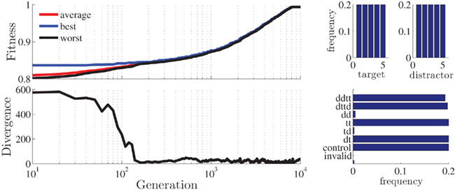
Figure 5. Statistics for the best stimulus-sequence generated with the setup for Schrobsdorff et al. (2007) study. Plotted are the fitness and divergence values as a function of generation (upper and lower left; log-scale) and histograms for target/distractor stimuli (upper right) and stimulus condition (lower right).

3.1.3 Example 3: Ihrke et al. (2011)

In a recent study, we conducted an NP experiment in which we implemented four different priming conditions, DT, TT, TD, and DD (Ihrke et al., 2011) that were to occur an equal number of times. There were 840 trials and 5 different stimuli. The results after 10000 iterations are optimal (ℱ = 1, Figure 6).

FIGURE 6

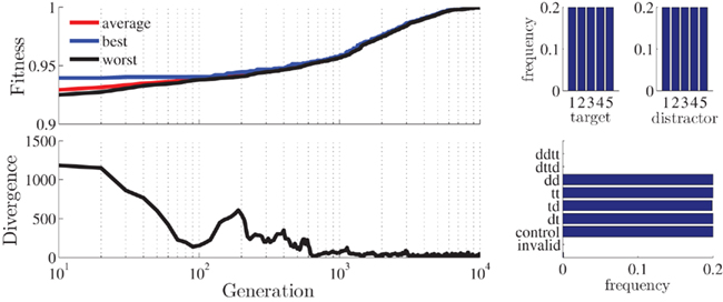
Figure 6. Statistics for the best stimulus-sequence generated with the setup for Ihrke et al. (2011) study. Plotted are the fitness and divergence values as a function of generation (upper and lower left; log-scale) and histograms for target/distractor stimuli (upper right) and stimulus condition (lower right).

3.2 Comparison with On-line Randomization

While it is more difficult to perform an on-line randomization for priming experiments than it is for paradigms without prime-probe relations, it is still possible when explicitly accounting for the inter-trial dependencies. To formulate a subroutine that can return the next stimuli given the preceding ones, it is convenient to use the terminology of Markov-chains. In these stochastic processes, the probability to be in a state at a given point in time depends only on the previous state. When associating the states with the presented stimuli, it is possible to create an algorithm for generating the next display which will converge to an optimal distribution of conditions and target/distractor stimuli in the limit of large number of trials. The details of this Markov-chain are described in the Appendix.

In Table 3, we present a comparison of stimulus-sequences generated using the GA and the on-line randomization for the three examples from the preceding section. The GA performs better in all cases. Because of the stochasticity of the on-line randomization, it can be expected that the overall quality of the method converges to optimal values with growing number of trials. In Figure 7, we present the score of the generated sequences using both the GA and the on-line randomization as a function of length (number of trials). While the GA finds an optimal solution independent of the number of trials in the sequence, the on-line solution approaches good results only for a large number of trials. The remaining gap between the two curves is a result of criterion C₃ in the calculation of the fitness-scores: Because the number of consecutive trials of the same experimental condition is punished in the GA but not in the on-line algorithm, the fitness of the on-line solution will always be lower than the GA-solution.

TABLE 3

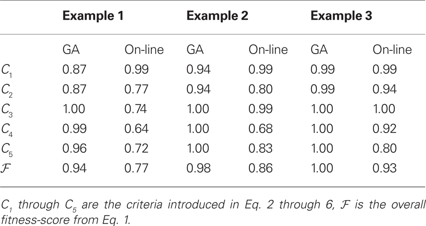
Table 3. Comparison of the genetic algorithm and the on-line approach for the presented examples (k = 6).

FIGURE 7

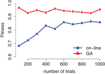
Figure 7. Performance of the genetic algorithm and the on-line strategy as a function of number of trials using the standard setup presented in Section 3. 1.1 (k = 6). While the GA produces optimal results also for lower number of trials, the fitness of the sequences from on-line randomization increases with the number of trials and saturates at a lower level than the GA-solution.

4 Discussion

Priming paradigms are widely applied in behavioral research and properly randomized trial sequences are an important basis for any successful priming experiment. Because the cross-trial dependency makes the use of on-line randomization more difficult and can even pose problems in manually designing randomized trial sequences, we developed a software that automatically generates suitable trial sequences based on a GA optimization strategy. GAs are argued to be particularly intuitive for behavioral researchers due to their similarity to biological evolution which lets the meaning of the parameters become transparent. A tool for manual tweaking of the generated sequences is provided as well. The software is suitable for priming tasks that vary from trial to trial on two independent dimensions. The program is hosted as an open-source project and is expected to evolve with the needs of experimentalists into a more general tool for trial-sequence generation. The software was designed to be extensible such that new requirements can be integrated in future versions with minimal programming effort.

4.1 Future Directions

We seek to extend the functionality of our program in several ways. Currently, if any experimental variation in addition to the priming conditions is desired, it must be added “by hand” to the generated trial-sequence using, e.g., a spreadsheet software. For example, recent studies have focused on response-repetitions in addition to the stimulus-repetitions covered by our software (e.g., Rothermund et al., 2005; Mayr et al., 2011). Randomization of the response-sequence in addition to the trial-sequence therefore includes additional inter-trial dependencies which must be uniformly distributed as well. We opt for the inclusion of such additional restrictions in future versions of our software.

Another important step is to increase the number of paradigms to which the program can be applied. Consider, for example, n-back tasks (e.g., Schmiedek, 2009): to support this task it is necessary to model inter-trial dependencies between trial i and trial i − n instead of only prime-probe dependencies. Our goal is to gradually approach a generality that will allow to model any such experimental requirements. This requires, however, a much more flexible formalism allowing the individual researcher to adapt the program to his needs. Currently, to adapt the software to different paradigms, programming skills are required: The fitness function as well as the stimulus-dependencies must be explicitly specified in the source-code. Later versions of our software are to include the possibility to specify any inter-trial dependencies on a variable number of dimensions.

Finally, we want to implement a measure for the randomness of a trial-sequence in order to avoid predictability in the recorded sequences. Potential candidates for such a measure are the Approximate Entropy (Pincus, 1991; Pincus and Kalman, 1997) or a derivate (e.g., Sample Entropy, Richman and Moorman, 2000) or the calculation of an entropy-measure for a minimal finite-state automaton fitted to the trial sequence (Cleeremans et al., 1989). However, there are several problems defining “predictability” by human subjects: First and foremost it is unclear what kind of sequential structure can be learned and used by human subjects. Studies on implicit sequence learning show that rather complex and stochastic structure can be exploited. Furthermore, due to the multivariate character of most trial sequences, it is not obvious whether only the sequential structure of each dimension or also cross-dependencies can be predicted. These considerations must be taken into account when designing a “measure of predictability” for trial sequences.

Conflict of Interest Statement

The authors declare that the research was conducted in the absence of any commercial or financial relationships that could be construed as a potential conflict of interest.

Acknowledgments

The first author acknowledges financial support by the Göttingen Graduate School for Neurosciences and Molecular Biosciences (GGNB). This work was supported by BMBF grant numbers 01GQ1005B and 01GQ0432. Discussions with Hecke Schrobsdorff, J. Michael Herrmann, Floran Schmiedek, and Marcus Hasselhorn are gratefully acknowledged.

Footnotes

1. ^Note that t_i and d_i refer to the ith element of the vectors t and d while t_i and d_i refer to the vectors of target and distractor in the ith genome.
2. ^The software depends on the freely available library for genetic algorithms GAlib by Wall (1999).
3. ^The runtime depends linearly on the three parameters: Doubling the number of generations/trials or the population size will approximately double the runtime as well.

References

Beasley, D., Bull, D., and Martin, R. (1993a). An overview of genetic algorithms: part 1, fundamentals. Univ. Comput. 15, 58–69.

Beasley, D., Bull, D., and Martin, R. (1993b). An overview of genetic algorithms: part 2, research topics. Univ. Comput. 15, 170–181.

Behrendt, J., Gibbons, H., Schrobsdorff, H., Ihrke, M., Herrmann, J. M., and Hasselhorn, M. (2010). Event-related brain potential correlates of identity negative priming from overlapping pictures. Psychophysiology 47, 921–930.

Pubmed Abstract | Pubmed Full Text

Boyer, M., Destrebecqz, A., and Cleeremans, A. (2005). Processing abstract sequence structure: learning without knowing, or knowing without learning? Psychol. Res. 69, 383–398.

Pubmed Abstract | Pubmed Full Text | CrossRef Full Text

Cleeremans, A., Servan-Schreiber, D., and McClelland, J. (1989). Finite state automata and simple recurrent networks. Neural Comput. 1, 372–381.

CrossRef Full Text

Cover, T. M., and Thomas, J. A. (2006). Elements of Information Theory, 2nd Edn. Hoboken, NJ: Wiley-Interscience.

Damian, M. F. (2000). Semantic negative priming in picture categorization and naming. Cognition 76, 45–55.

CrossRef Full Text

de Fockert, J. W., Mizon, G. A., and D’Ubaldo, M. (2010). No negative priming without cognitive control. J. Exp. Psychol. Hum. 36, 1333–1341.

CrossRef Full Text

Fox, E. (1995). Negative priming from ignored distractors in visual selection: a review. Psychon. Bull. Rev. 2, 145–173.

CrossRef Full Text

Frings, C., and Wentura, D. (2006). Strategy effects counteract distractor inhibition: negative priming with constantly absent probe distractors. J. Exp. Psychol. Hum. 32, 854–864.

CrossRef Full Text

Frings, C., and Wentura, D. (2008). Separating context and trial-by-trial effects in the negative priming paradigm. Eur. J. Cogn. Psychol. 20, 195–210.

CrossRef Full Text

Goldberg, D. (1989). Genetic Algorithms in Search, Optimization and Machine Learning Boston, MA: Addison-Wesley Longman Publishing Co., Inc.

Grison, S., and Strayer, D. L. (2001). Negative priming and perceptual fluency: more than what meets the eye. Percept. Psychophys. 63, 1063–1071.

Pubmed Abstract | Pubmed Full Text | CrossRef Full Text

Grison, S., Tipper, S. P., and Hewitt, O. (2005). Long-term negative priming: support for retrieval of prior attentional processes. Q. J. Exp. Psychol. 58, 1199–1224.

Ihrke, M. (2011). Gamixit. Available at: http://www.nld.ds.mpg.de/∼ihrke/gamixit

Ihrke, M., Behrendt, J., Schrobsdorff, H., Michael Herrmann, J., and Hasselhorn, M. (2011). Response-retrieval and negative priming. Exp. Psychol. 58, 154–161.

Pubmed Abstract | Pubmed Full Text

Kramer, A. F., and Strayer, D. L. (2001). Influence of stimulus repetition on negative priming. Psychol. Aging 16, 580–587.

Pubmed Abstract | Pubmed Full Text | CrossRef Full Text

Kristjánsson, á., and Driver, J. (2008). Priming in visual search: separating the effects of target repetition, distractor repetition and role-reversal. Vision Res. 48, 1217–1232.

CrossRef Full Text

Livesay, K., and Burgess, C. (1998). Mediated priming in high-dimensional semantic space: no effect of direct semantic relationships or co-occurrence. Brain Cogn. 37, 102–105.

Lorist, M., Boksem, M., and Ridderinkhof, K. (2005). Impaired cognitive control and reduced cingulate activity during mental fatigue. Cogn. Brain Res. 24, 199–205.

CrossRef Full Text

Lowe, D. (1998). Long-term positive and negative identity priming: evidence for episodic retrieval. Mem. Cognit. 26, 435–443.

Pubmed Abstract | Pubmed Full Text | CrossRef Full Text

May, C. P., Kane, M. J., and Hasher, L. (1995). Determinants of negative priming. Psychol. Bull. 118, 35–54.

Pubmed Abstract | Pubmed Full Text | CrossRef Full Text

Mayr, S., Möller, M., and Buchner, A. (2011). Evidence of vocal and manual event files in auditory negative priming. Exp. Psychol. 58, 353–360.

Pubmed Abstract | Pubmed Full Text

Milliken, B., Joordens, S., Merikle, P. M., and Seiffert, A. E. (1998). Selective attention: a reevaluation of the implications of negative priming. Psychol. Rev. 105, 203–229.

Pubmed Abstract | Pubmed Full Text | CrossRef Full Text

Papoulis, A., and Pillai, S. U. (2002). Probability, Random Variables and Stochastic Processes, 4th Edn. New York, NY: McGraw-Hill Higher Education.

Pincus, S. (1991). Approximate entropy as a measure of system complexity. Proc. Natl. Acad. Sci. U.S.A. 88, 2297.

Pubmed Abstract | Pubmed Full Text | CrossRef Full Text

Pincus, S., and Kalman, R. (1997). Not all (possibly)“random” sequences are created equal. Proc. Natl. Acad. Sci. U.S.A. 94, 3513.

Pubmed Abstract | Pubmed Full Text | CrossRef Full Text

R Development Core Team. (2010). R: A Language and Environment for Statistical Computing. Vienna: R Foundation for Statistical Computing.

Richman, J., and Moorman, J. (2000). Physiological time-series analysis using approximate entropy and sample entropy. Am. J. Physiol. 278, H2039.

Rothermund, K., Wentura, D., and De Houwer, J. (2005). Retrieval of incidental stimulus-response associations as a source of negative priming. J. Exp. Psychol. Learn. 31, 482–495.

CrossRef Full Text

Schmiedek, F. (2009). Interference and facilitation in spatial working memory: age-associated differences in lure effects in the N-back paradigm. Psychol. Aging 24, 203–210.

Pubmed Abstract | Pubmed Full Text | CrossRef Full Text

Schrobsdorff, H., Ihrke, M., Kabisch, B., Behrendt, J., Hasselhorn, M., and Herrmann, J. M. (2007). A computational approach to negative priming. Conn. Sci. 19, 203–221.

CrossRef Full Text

Stadler, M., and Neely, C. B. (1997). Effects of sequence length and structure on implicit serial learning. Psychol. Res. 60, 14–23.

CrossRef Full Text

Stadler, M. A. (1992). Statistical structure and implicit serial learning. J. Exp. Psychol. Learn. 18, 318–327.

CrossRef Full Text

Tipper, S. P. (1985). The negative priming effect: inhibitory priming by ignored objects. Q. J. Exp. Psychol. 37, 571–590.

Titz, C., Behrendt, J., Menge, U., and Hasselhorn, M. (2008). A reassessment of negative priming within the inhibition framework of cognitive aging: there is more in it than previously believed. Exp. Aging Res. 34, 340–366.

Pubmed Abstract | Pubmed Full Text | CrossRef Full Text

Visser, I., Raijmakers, M. E. J., and Pothos, E. M. (2009). Individual strategies in artificial grammar learning. Am. J. Psychol. 122, 293–307.

Pubmed Abstract | Pubmed Full Text

Wall, M. (1999). Galib. Available at: http://lancet.mit.edu/ga/

Appendix

On-line randomization for priming experiments

Since in priming experiments the dependency is only between prime and probe, it is possible to use an on-line randomization approach based on Markov-chains (for an introduction to Markov-chains, see Papoulis and Pillai, 2002). A Markov-chain is a stochastic process X_t that is characterized by the Markov-property: The probability distribution for trial t depends only on the previous outcome,

Because the condition in trial i depends only on trial i − 1 for priming experiments, it is possible to formulate this requirement in terms of a Markov-chain.

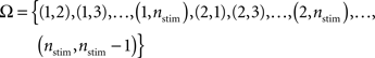
Given n_stim different stimuli, we formulate the state-space of a Markov-chain that consists of each possible individual display, i.e., each possible combination of two different stimuli (each display consists of target and distractor)

(trials in which target and distractor are identical are excluded, because they are considered to be invalid). The initial state is chosen randomly and the transition probabilities

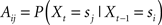
with s_i ∈ Ω are determined by the required distribution of priming conditions π_i, i ∈ Θ with Σ_iπ_i = 1. As before, this distribution is specified by the experimenter. Depending on which priming condition is chosen, the stimuli in the next display are restricted: In full repetition or full reversal trials, the stimuli will be the same as in the current trial (so there is only one possible transition). For all conditions with a single repetition, the number of possible stimuli for the probe is n_stim − 2, because one stimuli is fixed (the repeated one) and the other one can be any stimulus except the current target or distractor. In order to achieve a uniform distribution over the stimuli, the probability for the priming conditions in the probe is equally divided among all possible stimuli that realize this condition, such that A_ij = p_k = π_k/N_k for all i,j that result in priming condition k ∈ Θ. The number of possible transitions N_k per priming condition k is given in Table A1. For example, if the relative frequency of DT conditions in the trial sequence is to be π_DT = 0.2, then A_ij = 0.2/(n_stim − 2) for all i,j that will result in a DT condition. This will ensure that stimuli will be uniformly distributed in the limit of large number of trials. The process is illustrated in Figure A1.

FIGURE A1

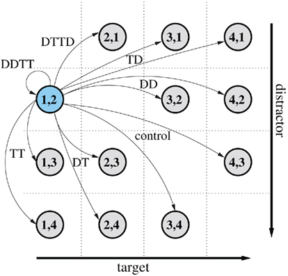
Figure A1. Illustration of a Markov-chain for n_stim = 4 different stimuli. The chain is currently in state (1,2) shown in blue (target 1 and distractor 2) and moves to a new stimulus combination with the transition probabilities A_ij as defined in the text.

TABLE A1

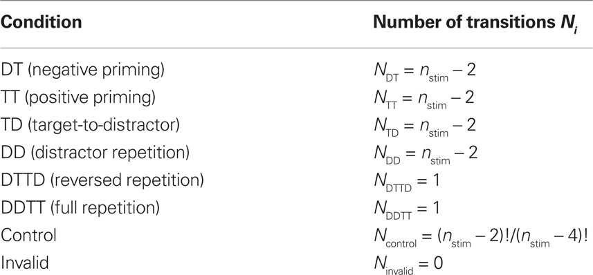
Table A1. Number of possible probe displays given a prime display when a specific priming condition is desired.

A script written in the R environment for statistical computation (R Development Core Team, 2010) that implements this idea is available from the website (Ihrke, 2011).