 Pablo Nájera
 Francisco José Abad
 Miguel A. Sorrel
- Department of Social Psychology and Methodology, Faculty of Psychology, Autonomous University of Madrid, Madrid, Spain
Cognitive diagnosis models (CDMs) allow classifying respondents into a set of discrete attribute profiles. The internal structure of the test is determined in a Q-matrix, whose correct specification is necessary to achieve an accurate attribute profile classification. Several empirical Q-matrix estimation and validation methods have been proposed with the aim of providing well-specified Q-matrices. However, these methods require the number of attributes to be set in advance. No systematic studies about CDMs dimensionality assessment have been conducted, which contrasts with the vast existing literature for the factor analysis framework. To address this gap, the present study evaluates the performance of several dimensionality assessment methods from the factor analysis literature in determining the number of attributes in the context of CDMs. The explored methods were parallel analysis, minimum average partial, very simple structure, DETECT, empirical Kaiser criterion, exploratory graph analysis, and a machine learning factor forest model. Additionally, a model comparison approach was considered, which consists in comparing the model-fit of empirically estimated Q-matrices. The performance of these methods was assessed by means of a comprehensive simulation study that included different generating number of attributes, item qualities, sample sizes, ratios of the number of items to attribute, correlations among the attributes, attributes thresholds, and generating CDM. Results showed that parallel analysis (with Pearson correlations and mean eigenvalue criterion), factor forest model, and model comparison (with AIC) are suitable alternatives to determine the number of attributes in CDM applications, with an overall percentage of correct estimates above 76% of the conditions. The accuracy increased to 97% when these three methods agreed on the number of attributes. In short, the present study supports the use of three methods in assessing the dimensionality of CDMs. This will allow to test the assumption of correct dimensionality present in the Q-matrix estimation and validation methods, as well as to gather evidence of validity to support the use of the scores obtained with these models. The findings of this study are illustrated using real data from an intelligence test to provide guidelines for assessing the dimensionality of CDM data in applied settings.
Introduction
The correct specification of the internal structure is arguably the key issue in the formulation process of a measurement model. Hence, it is not surprising that the determination of the number of factors has been regarded as the most crucial decision in the context of exploratory factor analysis (EFA; e.g., Garrido et al., 2013; Preacher et al., 2013). Since the very first proposals to address this issue, such as the eigenvalue-higher-than-one rule or Kaiser-Guttman criterion (Guttman, 1954; Kaiser, 1960), many methods have been developed for assessing the dimensionality in EFA. Despite the longevity of this subject of study, the fact that it is still a current research topic (e.g., Auerswald and Moshagen, 2019; Finch, 2020) is a sign of both its relevance and complexity.
In contrast to the vast research in the EFA framework, dimensionality assessment remains unexplored for other measurement models. This is the case of cognitive diagnosis models (CDMs). CDMs are restricted latent class models in which the latent variables or attributes are discrete, usually dichotomous. The popularity of CDMs has increased in the last years, especially in the educational field, because of their ability to provide a fine-grained information about the examinees' mastery or non-mastery of certain skills, cognitive processes, or competences (de la Torre and Minchen, 2014). However, CDM applications are not restricted to educational settings, and they have been employed for the study of psychological disorders (Templin and Henson, 2006; de la Torre et al., 2018) or staff selection processes (García et al., 2014; Sorrel et al., 2016).
A required input for CDMs is the Q-matrix (Tatsuoka, 1983). It has dimensions J items × K attributes, in which each q-entry (qjk) can adopt a value of 1 or 0, depending on whether attribute k is relevant to measure item j or not, respectively. Hence, the Q-matrix determines the internal structure of the test, and its correct specification is fundamental to obtain accurate structural parameter estimates and, subsequently, an accurate classification of examinees' latent classes or attribute profiles (Rupp and Templin, 2008; Gao et al., 2017). However, the Q-matrix construction process is usually conducted by domain experts (e.g., Sorrel et al., 2016). This process is subjective in nature and susceptible to specification errors (Rupp and Templin, 2008; de la Torre and Chiu, 2016). To address this, several Q-matrix estimation and validation methods have been proposed in the recent years with the aim of providing empirical support to its specification. On the one hand, empirical Q-matrix estimation methods rely solely on the data to specify the Q-matrix. For instance, Xu and Shang (2018) developed a likelihood-based estimation method, which aims to find the Q-matrix that shows the best fit while controlling for model complexity. Additionally, Wang et al. (2018) proposed the discrete factor loading (DFL) method, which consists in conducting an EFA and dichotomizing the factor loading matrix up to some criterion (e.g., row or column means). On the other hand, empirical Q-matrix validation methods aim to correct a provisional, potentially misspecified Q-matrix based on both its original specification and the data. For instance, the stepwise method (Ma and de la Torre, 2020a) is based on the Wald test to select the q-entries that are statistically necessary for each item, while the general discrimination index method (de la Torre and Chiu, 2016) and the Hull method (Nájera et al., 2020) aim to find, for each item, the simplest q-vector specification that leads to an adequate discrimination between latent classes. These methods serve as a useful tool for applied researchers, who can obtain empirical evidence of the validity of their Q-matrices (e.g., Sorrel et al., 2016).
Despite their usefulness, the Q-matrix estimation and validation methods share an important common drawback, which is assuming that the number of attributes specified by the researcher is correct (Xu and Shang, 2018; Nájera et al., 2020). Few studies have tentatively conducted either a parallel analysis (Robitzsch and George, 2019) or model-fit comparison (Xu and Shang, 2018) to explore the dimensionality of the Q-matrix. However, to the authors' knowledge, there is a lack of systematic studies on the empirical estimation of the number of attributes in CDMs. The main objective of the present research is precisely to compare the performance of a comprehensive set of dimensionality assessment methods in determining the number of attributes. The remaining of the paper is laid out as follows. First, a description of two popular CDMs is provided. Second, a wide selection of EFA dimensionality assessment methods is described. Third, an additional method for assessing the number of attributes in CDMs is presented. Fourth, the design and results from an exhaustive simulation study are provided. Fifth, real CDM data are used for illustrating the functioning of the dimensionality assessment methods. Finally, practical implications and future research lines are discussed.
The Dina and G-Dina Models
CDMs can be broadly separated into general and reduced, specific models. General CDMs are saturated models that subsume most of the reduced CDMs. They include more parameters and, consequently, provide a better model-data fit in absolute terms. As a counterpoint, their estimation is more challenging. Thus, reduced CDMs are often a handy alternative to applied settings because of their simplicity, which favors both their estimation and interpretation. Let denote by the number of required attributes for item j. Under the deterministic inputs, noisy “and” gate model (DINA; Junker and Sijtsma, 2001), which is a conjunctive reduced CDM, there are only two parameters per item regardless of : the guessing parameter (gj), which is the probability of correctly answering item j for those examinees that do not master, at least, one of the required attributes, and the slip parameter (sj), which is the probability of failing item j for those examinees that master all the attributes involved. The probability of correctly answering item j given latent class l is given by
where ηlj equals 1 if examinees in latent class l master all the attributes required by item j, and 0 otherwise.
The generalized DINA model (G-DINA; de la Torre, 2011) is a general CDM, in which the probability of correctly answering item j for latent class l is given by the sum of the main effects of the required attributes and their interaction effects (in addition to the intercept):
where is the reduced attribute profile whose elements are the required attributes for item j, δj0 is the intercept for item j, δjk is the main effect due to αk, is the interaction effect due to αk and , and is the interaction effect due to . Figure 1 depicts the probabilities of success of the four possible latent groups for an item requiring two attributes ( = 2) under the DINA and G-DINA models. For the DINA model, the probability of success for the latent group that masters all attribute is high (P(11) = 1 − sj = 1 − 0.2 = 0.8), while the probability of success for the remaining latent groups is very low (P(00) = P(10) = P(01) = gj = 0.1). For the G-DINA model, the baseline probability (i.e., intercept) is also very low (P(00) = δj0 = 0.1). The increment in the probability of success as a result of mastering the first attribute (P(10) = δj0 + δj1 = 0.1 + 0.25 = 0.35) is slightly lower than the one due to mastering the second attribute (P(01) = δj0 + δj2 = 0.1 + 0.35 = 0.45). Finally, although the interaction effect for both attributes is low (δj12 = 0.1), the probability of success for the latent group that masters both attributes is high because the main effects are also considered (P(11) = δj0 + δj1 + δj2 + δj12 = 0.1 + 0.25 + 0.35 + 0.1 = 0.80).
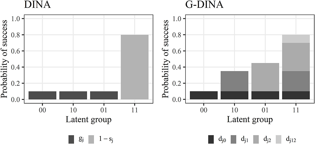
Figure 1. Illustration of item parameters and probabilities of success of the different latent groups for the DINA and G-DINA models involving 2 attributes (K = 2).
Dimensionality Assessment Methods
In the following, we provide a brief explanation of seven dimensionality assessment methods that were originally developed for determining the number of factors in EFA and will be explored in the present study.
Parallel Analysis
Parallel analysis (PA; Horn, 1965) compares the eigenvalues extracted from the sample correlation matrix (i.e., sample eigenvalues) with the eigenvalues obtained from several randomly generated correlation matrices (i.e., reference eigenvalues). The number of sample eigenvalues that are higher than the average of their corresponding reference eigenvalues is retained as the number of factors. The 95th percentile has also been recommended rather than the mean to prevent from over-factoring (i.e., overestimate the number of factors). However, no differences have been found in recent simulation studies between both cutoff criteria (Crawford et al., 2010; Auerswald and Moshagen, 2019; Lim and Jahng, 2019). Additionally, polychoric correlations have been recommended when working with categorical variables. Although no differences have been found for non-skewed categorical data, polychoric correlations perform better with skewed data (Garrido et al., 2013) as long as the reference eigenvalues are computed considering the univariate category probabilities of the sample variables by, for instance, using random column permutation for generating the random samples (Lubbe, 2019). Finally, different extraction methods have been used to compute the eigenvalues: principal components analysis (Horn, 1965), principal axis factor analysis (Humphreys and Ilgen, 1969), or minimum rank factor analysis (Timmerman and Lorenzo-Seva, 2011). The original proposal by Horn has consistently shown the best performance across a wide range of conditions (Garrido et al., 2013; Auerswald and Moshagen, 2019; Lim and Jahng, 2019). Simulation studies have shown the superiority of PA above other dimensionality assessment methods. Thus, it is usually recommended and considered the gold standard (Garrido et al., 2013; Auerswald and Moshagen, 2019; Lim and Jahng, 2019; Finch, 2020). As a flaw, PA tends to under-factor (i.e., underestimate the number of factors) in conditions with low factor loadings or highly correlated factors (Garrido et al., 2013; Lim and Jahng, 2019).
Minimum Average Partial
The minimum average partial (MAP; Velicer, 1976) method has also been recommended for determining the number of factors with continuous data (Peres-Neto et al., 2005). It is based on principal components analysis and the partial correlation matrix. The MAP method extracts one component at a time and computes the average of the squared partial correlations (MAP index). The MAP method relies on the rationale that extracting the first components, which explain most of the common variance, will result in a decrease of the MAP index. Once the relevant components have been partialled out, extracting the remaining ones (which are formed mainly by unique variance) will make the MAP index to increase again. The optimal number of components corresponds to the lowest MAP index. A variant where the MAP index is computed by averaging the fourth power of the partial correlation was proposed by Velicer et al. (2000). However, Garrido et al. (2011) recommended the use of the original squared partial correlations, in addition to polychoric correlations when categorical variables are involved. They found that MAP method performed poorly under certain unfavorable situations, such as low-quality items or small number of variables per factor, where the method showed a tendency to under-factor.
Very Simple Structure
The very simple structure (VSS; Revelle and Rocklin, 1979) method was developed with the purpose of providing the best interpretable factor solution, understood as the absence of cross-loadings. In this procedure, a loading matrix with K factors is first estimated and rotated. Then, a simplified factor loading matrix () is obtained, given a prespecified complexity v. Namely, the v highest loadings for each item are retained and the remaining loadings are fixed to zero. Then, the residual correlation matrix is found by
where R is the observed correlation matrix and Φk is the factor correlation matrix. Then, the VSS index is computed as
where and MSR are the average of the squared residual and observed correlations, respectively. The VSS index is computed for each factor solution, and the highest VSS corresponds to the number of factors to retain. The main drawback of the procedure is that the researcher must prespecify a common expected complexity for all the items, which is usually v = 1 (VSS1; Revelle and Rocklin, 1979). In a recent simulation study, the VSS method obtained a poor performance under most conditions, over-factoring with uncorrelated factors and under-factoring with highly correlated factors (Golino and Epskamp, 2017).
Dimensionality Evaluation to Enumerate Contributing Traits
The dimensionality evaluation to enumerate contributing traits (DETECT; Kim, 1994; Zhang and Stout, 1999; Zhang, 2007) method is a nonparametric procedure that follows two strong assumptions: first, a single “dominant” dimension underlies the item responses, and second, the residual common variance between the items follows a simple structure (i.e., without cross-loadings). The method estimates the covariances of item pairs conditioned to the raw item scores, which are used as a non-parametric approximation to the dominant dimension. If the data are essentially unidimensional, these conditional covariances will be close to zero. Otherwise, items measuring the same secondary dimension will have positive conditional covariances, and items measuring different secondary dimensions will have negative conditional covariances. The DETECT index is computed as
where P represents a specific partitioning of items into clusters, is the estimated conditional covariance between items j and j′, is the average of the estimated conditional covariances, and = 0 or 1 if items j and j′ are part of the same cluster or not, respectively. The method explores different number of dimensions and the one that obtains the highest DETECT index is retained. Furthermore, the method also provides which items measure which dimension. In a recent study, Bonifay et al. (2015) found that the DETECT method had a great performance at the population level, retaining the correct number of dimensions in 97% of the generated datasets with N = 10,000. As a limitation of the study, the authors only tested a scenario in which the generating model had no cross-loadings (i.e., simple structure).
Empirical Kaiser Criterion
The empirical Kaiser criterion (EKC; Braeken and van Assen, 2017) is similar to PA in that the sample eigenvalues are compared to reference eigenvalues to determine the number of factors to retain. Here, reference eigenvalues are derived from the theoretical sampling distribution of eigenvalues, which is a Marčenko-Pastur distribution (Marčenko and Pastur, 1967) under the null hypothesis (i.e., non-correlated variables). The first reference eigenvalue depends only on the ratio of test length to sample size, while the subsequent reference eigenvalues consider the variance explained by the previous ones. The reference eigenvalues are coerced to be at least equal to 1, and thus it cannot suggest more factors than the Kaiser-Guttman criterion would. In fact, EKC is equivalent to the Kaiser-Guttman criterion at the population level. EKC has been found to perform similarly to PA with non-correlated variables, unidimensional models, and orthogonal factors models, while it outperformed PA with oblique factors models and short test lengths (Braeken and van Assen, 2017). The performance of EKC with non-continuous data remains unexplored.
Exploratory Graph Analysis
EGA (Golino and Epskamp, 2017) is a recently developed technique that has emerged as a potential alternative for PA. EGA was first developed based on the Gaussian graphical model (GGM; Lauritzen, 1996), which is a network psychometric model in which the joint distribution of the variables is estimated by modeling the inverse of the variance-covariance matrix. The GGM is estimated using the least absolute shrinkage and selector operator (LASSO; Tibshirani, 1996), which is a penalization technique to avoid overfitting. Apart from EGA with GGM, Golino et al. (2020) recently proposed an EGA based on the triangulated maximally filtered graph approach (TMFG; Massara et al., 2016), which is not restricted to multivariate normal data. Regardless of the model (GGM or TMFG), in EGA each item is represented by a node and each edge connecting two nodes represents the association between the two items. Partial correlations are used for EGA with GGM, while any association measure can be used for EGA with TMFG. A strong edge between two nodes is interpreted as both items being caused by the same latent variable. A walktrap algorithm is then used to identify the number of clusters emerging from the edges, which will be the number of factors to retain. Furthermore, EGA also provides information about what items are included in what clusters, and clusters can be related to each other if their nodes are correlated. EGA with GGM seems to have an overall better performance than EGA with TMFG (Golino et al., 2020). EGA with GGM has been found to perform similarly to PA in most situations, with slightly worse results with low factor correlations, but better performance with highly correlated factors (Golino and Epskamp, 2017). On the other hand, EGA with TMFG tends to under-factor when there are many variables per factor or highly correlated factors (Golino et al., 2020).
Factor Forest
Factor forest (FF; Goretzko and Bühner, 2020) is an extreme gradient boosting machine learning model that was trained to predict the optimal number of factors in EFA. Specifically, the model estimates the probability associated to different factor solutions and subsequently suggests the number of factors with the highest probability. As opposed to the previously described dimensionality assessment methods, the FF is not based on any particular theoretical psychometric background, and its purpose is to make accurate predictions based on a combination of empirical results obtained from the training datasets. This is commonly referred to as the “black box” character of the machine learning models (Goretzko and Bühner, 2020). In the original paper, the authors trained the FF model using a set of 181 features (e.g., eigenvalues, sample size, number of variables, Gini-coefficient, Kolm measure of inequality) while varying the sample size, primary and secondary loadings, number of factors, variables per factor, and factor correlations, through almost 500,000 datasets. The data were generated assuming multivariate normality. The FF model obtained very promising results, correctly estimating the number of factors in 99.30% of the evaluation datasets. The Kolm measure of inequality and the Gini-coefficient were the most influential features on the predictions of the model. It is remarkable that some evaluation conditions were different from those used in the training stage. Thus, the FF model trained in Goretzko and Bühner (2020) for the EFA framework will be explored in the present paper.
Model-Fit Indices for Determining the Number of Attributes in CDM
All the aforementioned methods were developed with the purpose of assessing the number of factors in the EFA framework and, thus, their assumptions might not fit the nature of CDM data. Table 1 shows that some of the most important assumptions required by some of the methods might be usually violated when analyzing CDM data. There is, however, one additional procedure that can be applied to CDMs without any further assumptions: the model comparison approach based on model-fit indices. This approach has also been widely explored in EFA. Previous studies have shown that, even though the traditional cutoff points for some commonly used fit indices (e.g., CFI, RMSEA, SRMR) are not recommended for determining the number of factors (Garrido et al., 2016), the relative difference in fit indices between competing models might even outperform PA under some conditions, such as small loadings, categorical data (Finch, 2020), or orthogonal factors (Lorenzo-Seva et al., 2011). Additionally, Preacher et al. (2013) recommended to use AIC for extracting the number of factors whenever the goal of the research was to find a model with an optimal parsimony-fit balance, while they recommended RMSEA whenever the goal was to retain the true, generating number of factors.
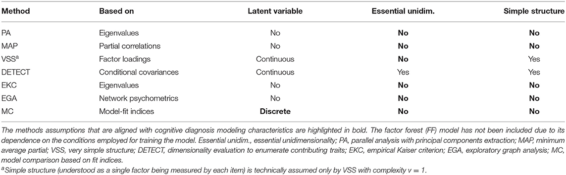
Table 1. Dimensionality assessment methods assumptions.
In the CDM framework, relative and absolute fit indices have been used to select the most appropriate Q-matrix specification. Regarding relative model-fit indices, Kunina-Habenicht et al. (2012) and Chen et al. (2013) found that Akaike's information criterion (AIC; Akaike, 1974) and Bayesian information criterion (BIC; Schwarz, 1978) perform really well at selecting the correct Q-matrix among competing matrices. In this vein, AIC and BIC always selected the correct Q-matrix when a three-attribute model was estimated for data generated from a five-attribute model, and vice versa (Kunina-Habenicht et al., 2012). Regarding absolute fit indices, Chen et al. (2013) proposed to inspect the residuals between the observed and predicted proportion correct of individual items (pj), between the observed and predicted Fisher-transformed correlation of item pairs (), and between the observed and predicted log-odds ratios of item pairs (). Specifically, they used the p-value associated to the maximum z-scores of pj, , and to evaluate absolute fit. While pj obtained very bad overall results, and performed appropriately at identifying both Q-matrix and CDM misspecification, with a tendency to be conservative.
The aforementioned studies pointed out that these fit indices are promising for identifying the most appropriate Q-matrix. However, further research is required to examine their systematic performance in selecting the most appropriate number of attributes across a wide range of conditions. The use of fit indices to select the most appropriate model among a set of competing models, from 1 to K number of attributes, requires the calibration of K CDMs, each of them requiring a specified Q-matrix. This task demands an unfeasible amount of effort if done by domain experts, but it is viable if done by empirical means. The idea of using an empirical Q-matrix estimation method to generate Q-matrices for different number of attributes and then compare their model-fit has been already suggested by Chen et al. (2015). Furthermore, the edina package (Balamuta et al., 2020a) of the R software (R Core Team, 2020) incorporates a function to perform a Bayesian estimation of a DINA model (Chen et al., 2018) with different number of attributes, selecting the best model according to the BIC. In spite of these previous ideas, the performance of fit indices in selecting the best model among different number of attributes has not been evaluated in a systematic fashion, including both reduced (e.g., DINA) and general (e.g., G-DINA) CDMs. More details about the specific procedure used in the present study for assessing the number of attributes using model comparison are provided in the Method section.
Goals of the Current Study
The main goal of the present study is to compare the performance of several dimensionality assessment methods in determining the generating number of attributes in CDM. Additionally, following the approach of Auerswald and Moshagen (2019), the combined performance of the methods is also evaluated to explore whether a more accurate combination rule can be obtained and recommended for applied settings. As a secondary goal, the effect of a comprehensive set of independent variables and their interactions over the accuracy of the procedures is systematically evaluated.
Table 1 provides the basis for establishing some hypotheses related to the performance of the methods. First, while CDMs are discrete latent variable models, most methods do not consider the existence of latent variables (PA with principal components extraction, MAP, EKC, EGA) or consider the existence of continuous latent variables (VSS, DETECT). The violation of this assumption might not be too detrimental, given that PA with component analysis violates EFA assumptions and is the current gold standard. On the other hand, both essential unidimensionality and simple structure assumptions are expected to have a great disruptive effect, since CDMs are usually highly multidimensional and often contain multidimensional items. Accordingly, VSS with v = 1 (VSS1) and DETECT are expected to perform poorly. Although VSS with complexity v > 1 is not technically assuming a simple structure (understood as a single attribute being measured by each item), its performance is still expected to be poor because of its stiffness and inability to adapt to the usual complex structure (i.e., items measuring a different number of attributes) of CDM items. Even though the remaining methods (i.e., PA, EKC, MAP, and EGA) do not assume a simple structure, their performance under complex structures remains mostly unexplored. Assessing the dimensionality of complex structures is expected to be more challenging compared to simple structures, in a similar fashion as correlated factors are more difficult to extract than orthogonal factors. The extent to which the performance of these methods is robust under complex structures is unknown. All in all, and considering the assumptions of each method, PA, EKC, MAP, and EGA, as well as the CDM model comparison approach based on fit indices (MC), are expected to perform relatively well, except for their idiosyncratic weakness conditions found in the available literature as previously described. Finally, the performance of FF is difficult to predict due to its dependency on the training samples. Even though no training samples were generated based on discrete latent variables in Goretzko and Bühner (2020), the great overall performance and generalizability of the FF model to conditions different from the ones used to train the model might extend to CDM data as well.
Methods
Dimensionality Estimation Methods
Eight different dimensionality estimation methods, with a total of 18 variants, were used in the present simulation study. The following text describes the specific implementation of each method.
Parallel Analysis
Four variants of PA were implemented as a function of the correlation matrix type (r = Pearson; ρ = tetrachoric) and the reference eigenvalue criterion (m = mean; 95 = 95th percentile): PArm, PAr95, PAρm, and PAρ95. All variants were implemented with principal components extraction and 100 random samples generated by random column permutation (Garrido et al., 2013; Lubbe, 2019). The sirt package (Robitzsch, 2020) was used to estimate the tetrachoric correlations for PA, as well as for the remaining methods that also make use of tetrachoric correlations.
Minimum Average Partial
MAP indices were based on the squared partial tetrachoric correlations computed with the psych package (Revelle, 2019). The maximum number of dimensions to extract was set to 9 (same for VSS, DETECT, and MC), so there was room for overestimating the number of attributes (the details of the simulation study are provided in the Design subsection).
Very Simple Structure
VSS was computed using tetrachoric correlations and the psych package. In addition to the most common VSS with complexity v = 1 (VSS1), VSS with complexity v = 2 (VSS2) was also explored.
Dimensionality Evaluation to Enumerate Contributing Traits
The DETECT index was computed using the sirt package, which uses the hierarchical Ward algorithm (Roussos et al., 1998) for clustering the items.
Empirical Kaiser Criterion
EKC was implemented by using tetrachoric correlations and the semTools package (Jorgensen et al., 2019).
Exploratory Graph Analysis
Two variants of EGA were implemented: EGA with GGM (EGAG) and EGA with TMFG (EGAT). The EGAnet package (Golino and Christensen, 2020) was employed for computing both variants.
Factor Forest
The R code published by Goretzko and Bühner (2020) at Open Science Framework1 was used for the implementation of the FF model trained in their original paper. With this code, FF can recommend between one and eight factors to retain.
Model Comparison Based on Fit Indices
The MC procedure was implemented varying the number of attributes from 1 to 9 as follows. First, the DFL Q-matrix estimation method (Wang et al., 2018) using Oblimin oblique rotation, tetrachoric correlations, and the row dichotomization criterion was used to specify the initial Q-matrix, and the Hull validation method (Nájera et al., 2020) using the PVAF index was then implemented to refine it and provide the final Q-matrix. Second, a CDM was fitted to the data using the final Q-matrix with the GDINA package (Ma and de la Torre, 2020b). The CDM employed to fit the data was the same as the generating CDM (i.e., DINA or G-DINA). This resulted in a set of nine competing models varying in K. Third, the models were alternatively compared with the AIC, BIC, and fit indices. For the AIC and BIC criteria, the model with the lowest value was retained. Regarding , the number of items with some significant pair-wise residual (after using Bonferroni correction at the item-level) was counted. Then, the most parsimonious model with the lowest count was retained. The MC procedure with AIC, BIC, or will be referred to as MCAIC, MCBIC, and MCr, respectively. Given that the MC procedures rely on empirically specified Q-matrices, their performance will greatly depend on the quality of such Q-matrices. Even though the DFL and Hull methods have provided good results in previous studies, their combined performance should be evaluated to examine the quality of their suggested Q-matrices. For this reason, the proportion of correctly specified q-entries was computed for the estimated (i.e., DFL) and validated (i.e., DFL and Hull) Q-matrices (more details are provided in the Dependent variables subsection). The further the DFL and Hull methods are from a perfect Q-matrix recovery, the greater the room for improvement for the MC procedures. In this vein, the set of nine competing models (using DFL and Hull) were additionally compared to the model using the generating Q-matrix, with the purpose of providing an upper-limit performance for the MC methods when the Q-matrix is perfectly recovered. The results of these comparisons will be referred to as MCAIC−G, MCBIC−G, and MCr−G.
Design
Table 2 shows the factors (i.e., independent variables) used in the simulation study: number of attributes (K), item quality (IQ), sample size (N), ratio of number of items to attribute (JK), underlying correlation among the attributes (AC), and attribute thresholds (AT). The levels of each factor were selected in pursuit of representativeness of varying applied settings. For instance, the most common number of attributes (K) seen in applied studies is 4 (Sessoms and Henson, 2018), while 5 is the most usual value in simulation studies (e.g., de la Torre and Chiu, 2016; Ma and de la Torre, 2020a). The levels selected for item quality (IQ), sample size (N), and ratio of number of items to attribute (JK) are also considered as representative of applied settings (Nájera et al., 2019; Ma and de la Torre, 2020a). Regarding the attribute correlations, some applied studies have obtained very high attribute correlation coefficients, up to 0.90 (Sessoms and Henson, 2018). It can be argued that these extremely high correlations may be indeed a consequence of overestimating the number of attributes, where one attribute has been split into two or more undifferentiated attributes. For this reason, we decided to use AC levels similar to those used in EFA simulation studies (e.g., Garrido et al., 2013). Additionally, different attribute thresholds (AT) levels were included to generate different degrees of skewness in the data, given its importance in the performance of dimensionality assessment methods (Garrido et al., 2013). Finally, both a reduced CDM (i.e., DINA) and a general CDM (i.e., G-DINA) were used to generate data. A total of 972 conditions, resulting from the combination of the factor levels, were explored.
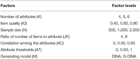
Table 2. Summary of the factors explored in the simulation study.
Data Generation
One hundred datasets were generated per condition. Examinees' responses were generated using either the DINA or G-DINA model. Attribute distributions were generated using a multivariate normal distribution with mean equal to 0 for all attributes. All underlying attribute correlations were set to the corresponding AC condition level. Attribute thresholds, which are used to dichotomize the multivariate normal distribution to determine the mastery or non-mastery of the attributes, were generated following an equidistance sequence of length K between –AT and AT. This results in approximately half of the attributes being “easier” (i.e., higher probabilities of attribute mastery) and the other half being “more difficult” (i.e., lower probabilities of attribute mastery). For instance, for AT = 0.50 and K = 5, the generating attributes thresholds were {−0.50, −0.25, 0, 0.25, 0.50}.
Item quality was generated by varying the highest and lowest probabilities of success, which correspond to the latent classes that master all, P(1), and none, P(0), of the attributes involved in an item, respectively. These probabilities were drawn from uniform distributions as follows: P(0)~U(0, 0.20) and P(1)~U(0.80, 1) for high-quality items, P(0)~U(0.10, 0.30) and P(1)~U(0.70, 0.90) for medium-quality items, and P(0)~U(0.20, 0.40) and P(1)~U(0.60, 0.80) for low-quality items. The expected value for the item quality across the J items is then 0.80, 0.60, and 0.40 for high, medium, and low-quality items, respectively. For the G-DINA model, the probabilities of success for the remaining latent classes were simulated randomly, with two constraints. First, a monotonicity constraint on the number of attributes was applied. Second, the sum of the δ parameters associated to each attribute was constrained to be higher than 0.15 to ensure the relevance of all the attributes (Nájera et al., 2020).
The Q-matrices were generated randomly with the following constraints: (a) each Q-matrix contained, at least, two identity matrices; (b) apart from the identity matrices, each attribute was measured, at least, by another item; (c) the correlation between attributes (i.e., Q-matrix columns) was lower than 0.50; (d) the proportion of one-, two-, and three-attribute items was set to 0.50, 0.40, and 0.10. Constrains (a) and (b) are in line with the identifiability recommendations made by Xu and Shang (2018). Constrain (c) ensures non overlapping attributes. Finally, constrain (d) was based on the proportion of items measuring one-, two-, and three-attributes encountered in previous literature. We examined the 36 applied studies included in the literature revision by Sessoms and Henson (2018) and extracted the complexity of the q-vectors from the 17 studies that reported the Q-matrix (see Table 3). The reason why we used a higher proportion of one-attribute items was to preserve constrain a). For instance, in the condition of JK = 4, at least 50% of one-attribute items are required to form two identity matrices.
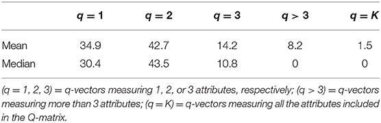
Table 3. Complexity of q-vectors in applied studies (percentages).
Dependent Variables
Four dependent variables were used to assess the accuracy of the dimensionality assessment methods. The hit rate (HR) was the main dependent variable, computed as the proportion of correct estimates:
where I is the indicator function, is the recommended number of attributes, K is the generating number of attributes, and R is the number of replicates per condition (i.e., 100). A HR of 1 indicates a perfect accuracy, while an HR of 0 indicates complete lack of accuracy. Additionally, given that a model selection must be done according to both empirical and theoretical criteria, it is a recommended approach to examine alternative models to the one suggested by a dimensionality assessment method (e.g., Fabrigar et al., 1999). The close hit rate (CHR) was assessed to explore the proportion of times that a method recommended a number of attributes close to the generating number of attributes:
Finally, the mean error (ME) and root mean squared error (RMSE) were explored to assess the bias and inaccuracy of the methods:
A ME of 0 indicates lack of bias, while a negative or positive ME indicates a tendency to underestimate or overestimate the number of attributes, respectively. It is important to note that an ME close to 0 can be achieved either by an accurate method, or by a compensation of under- and overestimation. On the contrary, RMSE can only obtain positive values: the further from 0, the greater the inaccuracy of a method.
Univariate ANOVAs were conducted to explore the effect of the factors on the performance of each method. The dependent variables for the ANOVAs were the hit rate, close hit rate, bias, and absolute error, which correspond to the numerators of Equations (6)–(9) (i.e., HR, CHR, ME, and RMSE at the replica-level), respectively. Note that the RMSE computed at the replica level is the absolute error (i.e., ). Effects with a partial eta-squared () higher than 0.060 and 0.140 were considered as medium and large effects, respectively (Cohen, 1988).
In order to explore the performance of the combination rules (i.e., two or more methods taken together), the agreement rate (AR) was used to measure the proportion of conditions under which a combination rule recommended the same number of attributes, while the agreement hit rate (AHR) was used to measure the proportion of correct estimations among those conditions in which an agreement has been achieved:
where and are the recommended number of attributes by any two different methods. Note that these formulas can be easily generalized for more than two methods. Both a high AR and AHR are required for a combination rule to be satisfactory, since this indicates that it will be accurate and often applicable (Auerswald and Moshagen, 2019).
Finally, for the MC methods, when the model under exploration had the same number of attributes as the generating number of attributes, the Q-matrix recovery rate (QRR) was explored to assess the accuracy of the DFL and Hull methods. Specifically, it reflects the proportion of correctly specified q-entries. A QRR of 1 indicates perfect recovery. The higher the QRR, the closer the methods based on model-fit indices (e.g., MCAIC) should be to their upper-limit performance (e.g., using the generating Q-matrix as in MCAIC−G). All simulations and analyses were conducted using the R software. The data were simulated using the GDINA package. The codes are available upon request.
Results
Before describing the main results, the results for the QRR are detailed. The overall QRR obtained after implementing both the DFL and Hull method was 0.949. The lowest and highest QRR among the factor levels were obtained with IQ = 0.40 (QRR = 0.890) and IQ = 0.80 (QRR = 0.985), respectively. These results are consistent with Nájera et al. (2020). The DFL method alone (i.e., before validating the Q-matrix with the Hull method) led to a good overall accuracy (QRR = 0.939). However, despite this high baseline, the Hull method led to a QRR improvement across all factor levels (ΔQRR = [0.005, 0.013]).
Table 4 shows the overall average results, across all conditions, for all the variants and dependent variables considered. The four PA variants, FF, and MCAIC performed reasonably well, with a HR > 0.700 and a CHR > 0.900. EGAG also obtained a high CHR (CHR = 0.918), but a much lower HR (HR = 0.576). The highest HR was obtained by PArm (HR = 0.829), while the highest CHR was provided by MCAIC (CHR = 0.954). Congruently with these results, the PA variants, FF, MCAIC, and EGAG showed a low RMSE (RMSE <1), being the MCAIC the method with the lowest error (RMSE = 0.633). The remaining methods (i.e., MAP, VSS1, VSS2, DETECT, EKC, EGAT, MCBIC, and MCr) obtained a poorer performance (HR ≤ 0.682 and CHR ≤ 0.853). Regarding the bias, most methods showed a tendency to underestimate the number of attributes, especially MAP, VSS1, and EGAT (ME ≤ −0.831). On the contrary, EKC and DETECT showed a tendency to overestimate the number of attributes (ME ≥ 1.043). Among the methods with low RMSE, FF (ME = −0.191), PArm (ME = −0.144), and, especially, MCAIC (ME = 0.010), showed a very low bias. Finally, the MC methods that rely on the generating Q-matrix (i.e., MCAIC−G, MCBIC−G, MCr−G) generally provided good results, outperforming their corresponding MC method. Specifically, MCAIC−G obtained the highest overall accuracy (HR = 0.886; CHR = 0.975; RMSE = 0.458).
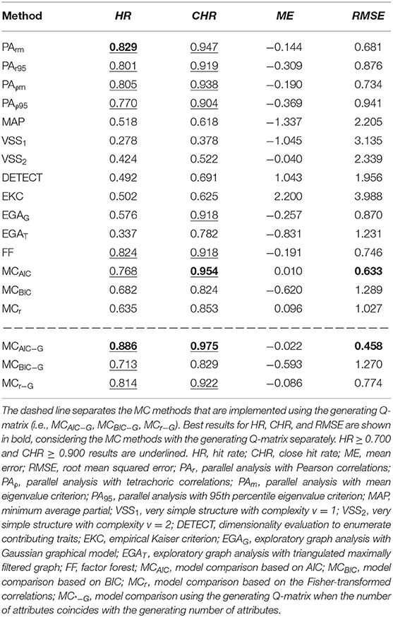
Table 4. Overall performance for all dimensionality estimation methods.
Table 5 shows the results for the methods that obtained the best overall performance as indicated by CHR > 0.900 (i.e., PArm, EGAG, FF, and MCAIC) across the factor levels. Only PArm is shown among the PA variants because their results were congruent and PArm obtained the better overall performance. In addition to these methods, the MCAIC−G is also included to provide a comparison with MCAIC. The results from Table 5 can be easier interpreted by inspecting the main effect size values obtained in the ANOVAs (see Table 6). These main effects offer a proper summary of the results since only one interaction effect, which will be described below, was relevant ( > 0.140).
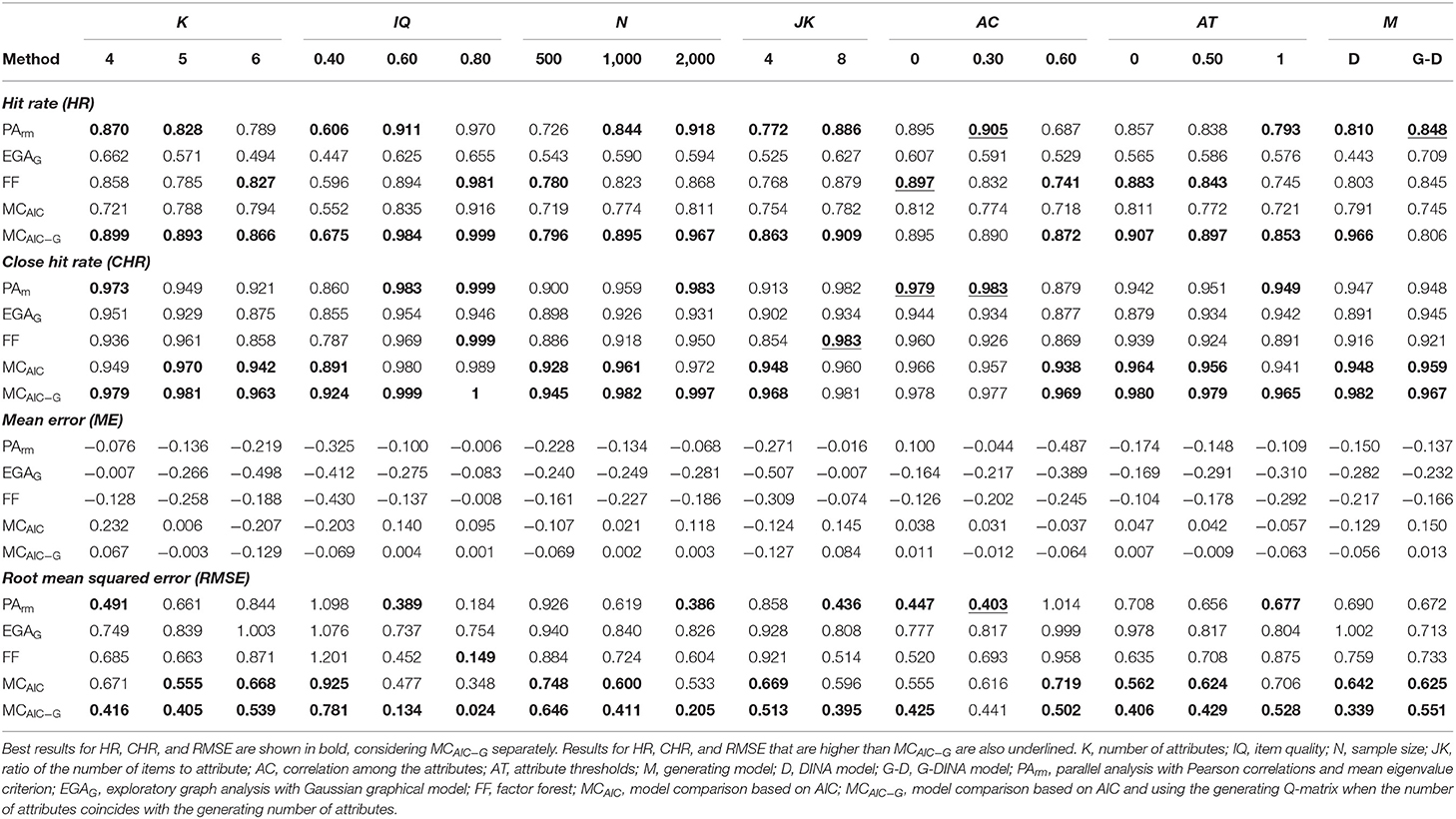
Table 5. Performance of the best methods by factor level.
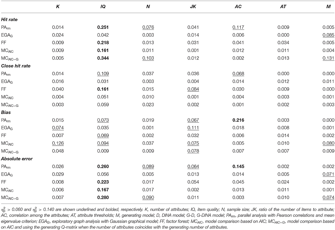
Table 6. Univariate ANOVAs main effect size values ().
Regarding the hit rate, IQ was the factor that most affected all the methods ( ≥ 0.161), except for EGAG. These methods performed very accurately with IQ = 0.80 (HR ≥ 0.916), but poorly with IQ = 0.40 (HR ≤ 0.675). Other factors obtained a medium effect size for one specific method. EGAG was affected by M, obtaining a higher accuracy with the G-DINA model (HR= 0.709) than with the DINA model (HR = 0.443). On the other hand, PArm was affected by N and AC. PArm obtained the highest HR in most conditions, especially with large sample sizes (N = 2000), but was negatively affected by high correlations among the attributes (AC = 0.60). In the cases in which PArm was not the best performing method, the FF obtained the highest accuracy. FF obtained the biggest advantage in comparison to the other methods under N = 500 (ΔHR = 0.054). Results for the RMSE showed a very similar pattern to those from HR. The most notable difference was that MCAIC obtained the lowest RMSE under most conditions, especially AC = 0.60 (|ΔRMSE| = 0.239). On the contrary, PArm showed a smaller error with lower attribute correlations, especially AC = 0.30 (|ΔRMSE| = 0.213).
The close hit rate of the methods was more robust than the HR to the different simulation conditions. Only PArm and, especially, FF were affected by IQ. PArm was also affected by AC, and FF by JK. The CHR of both EGAG and MCAIC remained stable across the factor levels. The highest CHR was obtained by MCAIC in most conditions, obtaining the biggest advantage under AC = 0.60 (ΔCHR = 0.059). PArm and FF provided the highest CHR in those conditions in which MCAIC did not obtain the best result.
With respect to the bias (i.e., ME), Table 6 shows that the only large effect was observed for AC on PArm. However, there was a relevant effect for the interaction between AC and IQ ( = 0.194). This was the only interaction with a large effect among all the ANOVAs. Namely, the strong tendency to underestimate seen for PArm under AC = 0.60 was mainly due to IQ = 0.40. Thus, under IQ = 0.40, PArm showed a strong tendency to underestimate when AC = 0.60 (ME = −1.108), but a slight tendency to overestimate when AC = 0 (ME = 0.258). With IQ ≥ 0.60 and AC ≤ 0.30, PArm obtained a low bias (ME ≤ |0.055|). Apart from this interaction, other factors with relevant effect sizes were: a) K, which had an effect on EGAG and MCAIC; b) IQ, with an effect on PArm, FF, and MCAIC; and c) JK, which had an effect on PArm, EGAG, and MCAIC. In general, the most demanding levels of these factors (i.e., K = 6, IQ = 0.40, JK = 4) led to an underestimation tendency for the methods. Finally, while PArm, EGAG, and FF showed a negative bias (i.e., ME <0) across almost all conditions, MCAIC showed a positive bias (i.e., ME > 0) under several conditions, especially K = 4 and the G-DINA model (ME ≥ 0.150).
Finally, MCAIC−G performed the best under almost all conditions and dependent variables, with the only exception of AC ≤ 0.30 and G-DINA generated data, where PArm obtained slightly better results. As expected, MCAIC−G outperformed MCAIC under all conditions. The ANOVA effects were similar for both methods. One of the main differences is that the HR of MCAIC−G was more affected by the sample size (a steeper HR improvement as N increased) and the generating model (performing comparatively better under the DINA model). On the other hand, the ME of MCAIC−G was more robust under different levels of K and M.
Table 7 shows the results for the combination rules split by sample size. VSS1, VSS2, DETECT, EKC, and EGAT are not included because they were not usually consistent with any other method (i.e., AR <0.50). Both the AR and the AHR tended to increase as the sample size increased. As expected from the results above, the best performing combination rules were mainly formed by PA (especially PArm), FF, and MC (especially MCAIC). The combination rule formed by PArm and FF obtained arguably the best balance between agreement and accuracy (AR ≥ 0.70; AHR ≥ 0.923), while FF and MCAIC obtained a higher accuracy with a slightly lower agreement (AR ≥ 0.65; AHR ≥ 0.953). The best accuracy was obtained by the combination rule formed by MCAIC and MAP (AHR ≥ 0.980), although at the cost of a lower agreement (AH ≈ 0.46). In addition to these two-method combination rules, the performance of the three best methods (i.e., PArm, FF, and MCAIC) taken together was also explored. This combination rule showed a very high overall accuracy while keeping an AR > 0.50. Specifically, for N = 500, 1000, and 2000, it obtained AHR (AR) = 0.976 (0.57), 0.985 (0.65), and 0.992 (0.70), respectively.
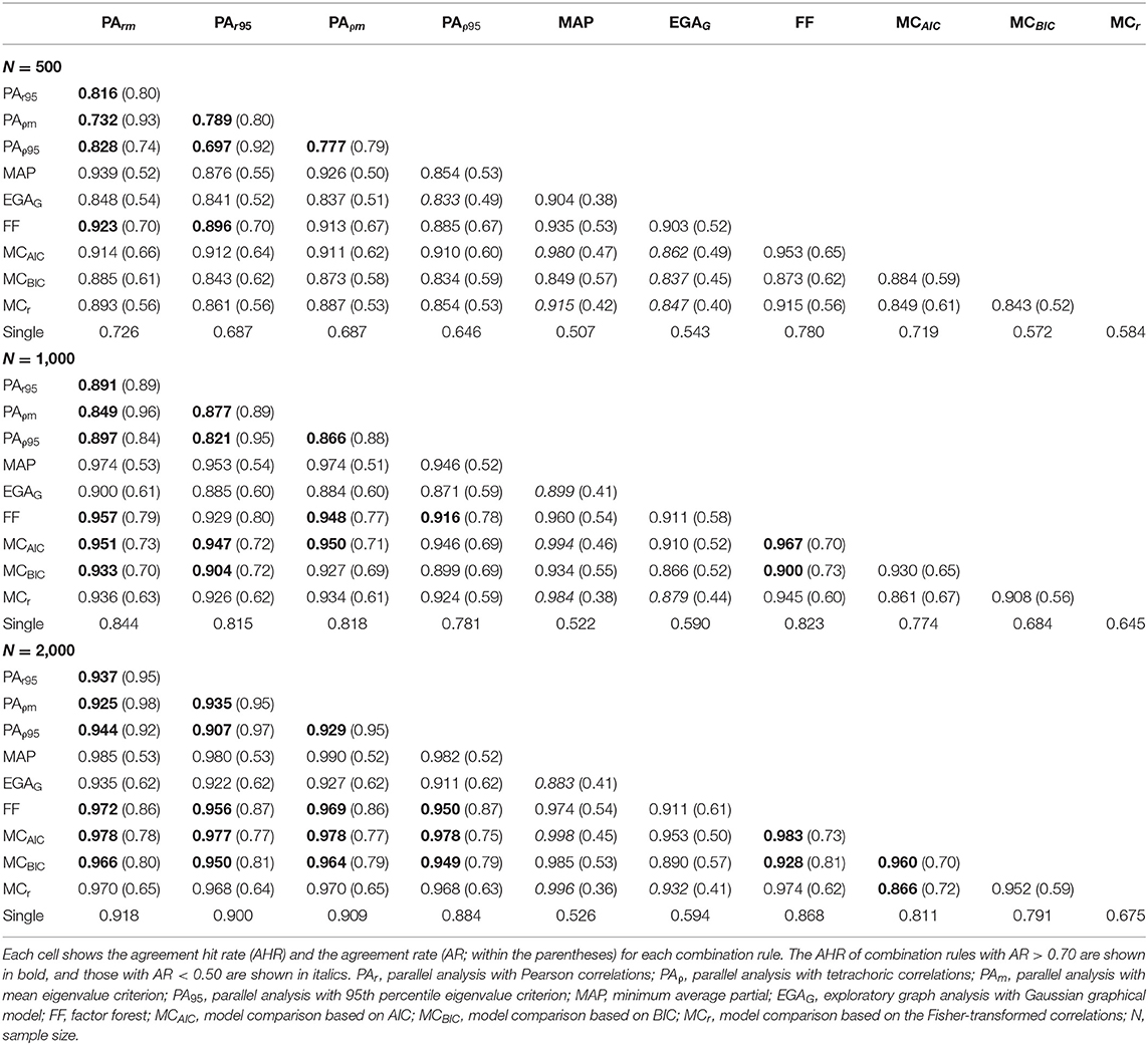
Table 7. Performance of the combination rules by sample size.
Real Data Example
Real data were analyzed to illustrate the performance of the dimensionality estimation methods explored in the simulation study. This section can be also understood as an illustration of how to approach the problem of determining the number of attributes in applied settings. The data employed for this example was previously analyzed by Chen et al. (2020). The dataset consists of dichotomous responses from 400 participants to 20 items from an intelligence test. Each item consists of nine matrices forming a 3 rows × 3 columns disposition, in which the ninth matrix (i.e., the lower right) is missing. Participants must select the missing matrix out of eight possible options. There are no missing data. The dataset is available at the edmdata package (Balamuta et al., 2020b) and item definitions can be found at Open Psychometrics.2 Chen et al. (2020) defined four attributes involved in the test: (a) learn the pattern from the first two rows and apply it to the third row, (b) infer the best overall pattern from the whole set of matrices, (c) recognize that the missing matrix is different from the given matrices (e.g., applying rotations or stretching), and (d) recognize that the missing matrix is exactly as one of the given matrices. The authors did not explicitly define a Q-matrix for this dataset because they focused on the exploratory estimation of the item parameters. However, they described a procedure to derive a Q-matrix from the item parameter estimates by dichotomizing the standardized coefficients related to each attribute (Chen et al., 2020, pp. 136). This original Q-matrix, which is here referred to as QO, is shown in Figure 2.
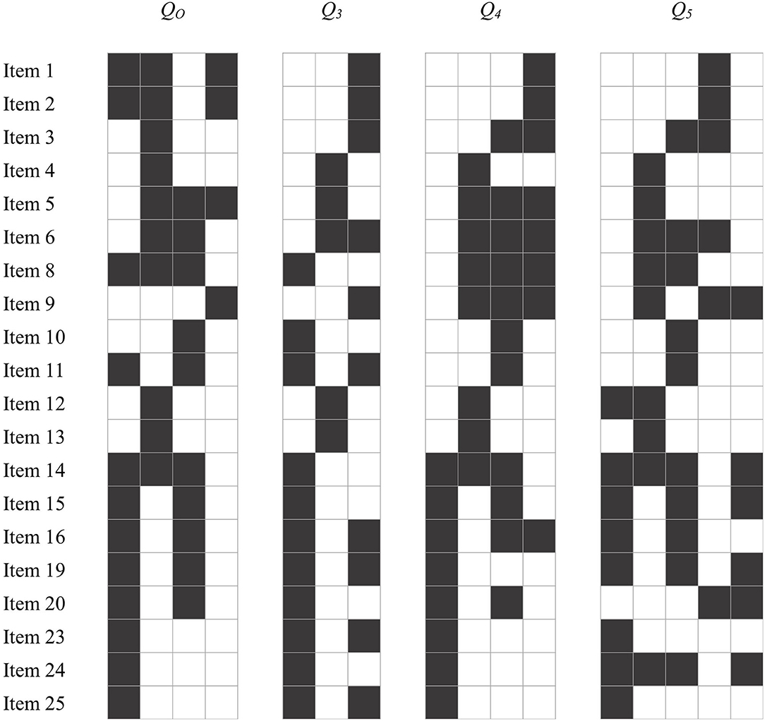
Figure 2. Q-matrices of the real data example. White cells represent qjk = 0 and black cells represent qjk = 1. QO is the Q-matrix from Chen et al. (2020); Q3 to Q5 are the suggested Q-matrices by DFL and Hull methods from 3 to 5 attributes.
According to the findings from the simulation study, the following steps are recommended to empirically determine the number of attributes in CDM data: (a) if PArm, FF, and MCAIC agree on their suggestion, retain their recommended number of attributes; (b) if any two of these methods agree, retain their recommended number of attributes; (c) if none of these methods agree, explore the recommended number of attributes by those that suggest a similar (i.e., ±1) number of attributes; (d) if these methods strongly disagree, explore the recommended number of attributes by each of them. Constructing several Q-matrices is a very challenging and time-consuming process for domain experts; thus, the Q-matrices suggested by the DFL and Hull methods (which are already used to implement the MC methods), can be used as a first approximation. Domain experts should be consulted to contrast the interpretability of these Q-matrices.
All the dimensionality assessment methods included in the simulation study were used to assess the number of attributes of the dataset. Their recommendations were as follows: 1 attribute was retained by MAP and VSS1; 2 attributes by PAρ95, PAρm, VSS2, and EGAT; 3 attributes by PArm, PAr95, and MCBIC; 4 attributes by EGAG, MCAIC, and MCr; 5 attributes by EKC and FF; and 8 attributes by DETECT. In accordance with the simulation study results, MAP, VSS1, and EGAT, which showed a tendency to underestimate, suggested a low number of attributes, while DETECT, which showed a strong tendency to overestimate, suggested the highest number of attributes.
Following the previously described guidelines, we focused on the recommendations of PArm, MCAIC, and FF (i.e., 3, 4, and 5 attributes, respectively). Step c of the guidelines apply to this case because none of the methods agreed on their suggestion, but PArm and MCAIC, as well as MCAIC and FF, recommended a close number of attributes. Thus, we explored solutions from 3 to 5 attributes in terms of model fit. A G-DINA model was fitted using each of the Q-matrices from 3 to 5 attributes (Q3-Q5) suggested by the DFL and Hull methods (see Figure 2). Additionally, QO was also used to fit a G-DINA model for comparison purposes. Table 8 shows the fit indices for each model. Overall, Q4 obtained the best model fit. This result is in agreement with the number of attributes defined by Chen et al. (2020). Thus, a solution with four attributes was considered the most appropriate. The differences between Q4 and QO were not very pronounced: 81.25% of the q-entries were the same for both matrices. In an applied study in which no original Q-matrix had been prespecified, Q4 could be used as a starting point for domain experts to achieve a Q-matrix specification that provides both good fit and theoretical interpretability.
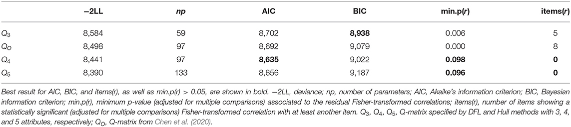
Table 8. Model-fit for the real data illustration Q-matrices.
Discussion
The correct specification of the Q-matrix is a prerequisite for CDMs to provide accurate attribute profile classifications (Rupp and Templin, 2008; Gao et al., 2017). Because the Q-matrix construction process is usually conducted by domain experts, many Q-matrix validation methods have been recently developed with the purpose of empirically evaluating the decisions made by the experts. Additionally, empirical methods to specify the Q-matrix directly from the data (i.e., Q-matrix estimation methods), without requiring a previously specified one, have been also proposed. The problem with the Q-matrix estimation and validation methods proposed so far is that they do not question the number of attributes specified by the researcher. The assumption of known dimensionality has not been exhaustively explored in the CDM framework. This contrasts with the vast literature on dimensionality assessment methods in the factor analysis framework, where this problem is considered of major importance and has received a high degree of attention (e.g., Garrido et al., 2013; Preacher et al., 2013). All in all, the main goal of the present study was to explore the performance of several dimensionality assessment methods from the available literature in determining the number of attributes in CDMs. A comprehensive simulation study was conducted with that purpose.
Results from the simulation study showed that some methods available can be considered suitable for assessing the dimensionality of CDMs. Namely, parallel analysis with principal components and random column permutation (i.e., PA), the machine learning factor forest model (i.e., FF), and using the AIC fit index to compare CDMs with different number of attributes (i.e., MCAIC) obtained high overall accuracies (HR ≥ 0.768). PA with Pearson correlations and mean eigenvalue criterion (i.e., PArm) obtained the highest overall accuracy, while MCAIC obtained the best close accuracy, considering a range of ±1 attribute around the generating number of attributes. Item quality was found to be the most relevant simulation factor, severely affecting the performance of PArm, FF, and MCAIC. Thus, the percentage of correct estimates varied from around 60% with low-quality items to more than 90% with high-quality items. Apart from item quality, PArm was also affected by the sample size and the correlation among the attributes, showing a bad performance with highly correlated attributes. These results are in line with previous studies (e.g., Garrido et al., 2013; Lubbe, 2019). MCAIC and, especially, FF, were more robust to the different explored conditions (other than item quality). However, it should be noted that, unlike PArm and FF (which consistently tended to underestimate the number of attributes under almost all conditions), MCAIC bias might show a slightly under- or overestimation tendency depending on the number of attributes, item quality, ratio of number of items to attribute, and generating model.
The remaining methods (i.e., MAP, VSS1, VSS2, DETECT, EKC, EGAG, EGAT, MCBIC, and MCr) obtained an overall poor performance, and thus their use cannot be recommended for the assessment of CDM data dimensionality. Of these methods, DETECT and EKC showed a heavy tendency to overestimate. Even though EKC was expected to perform better, it was observed that the first reference eigenvalue was usually very high, leaving the remaining ones at low levels. These resulted in the EKC often performing identically to what the Kaiser-Guttman criterion would (which is known for its tendency to overestimate the number of dimensions). On the other hand, MAP, VSS1, EGAT, and MCBIC showed a strong tendency to underestimate. Even though a higher performance was expected for MAP and EGAT, their underestimation tendency is aligned with previous findings (Garrido et al., 2011; Golino et al., 2020). As for the MC methods, while both AIC and BIC have shown good results in selecting the correct Q-matrix among competing misspecified Q-matrices (Kunina-Habenicht et al., 2012; Chen et al., 2013), it is clear that the higher penalization that BIC applies compared to AIC is not appropriate for the dimensionality assessment problem. Finally, EGAG was the only remaining method that obtained a good performance in terms of close hit rate. However, its overall hit rate was low, especially due to its poor performance when the generating model was the DINA model.
Although the influence of the generating model was most noticeable for EGAG, most dimensionality assessment methods from the EFA framework performed worse under the DINA model than under the G-DINA model. These results might be due to the non-compensatory nature of the DINA model, in which the relationship between the number of mastered attributes and the probability of correctly answering an item clearly deviates from being linear (in a more pronounced way that under the G-DINA model, as illustrated in Figure 1). A greater depart from linearity might produce a greater disruption to the performance of all the methods that are based on correlations (e.g., PA, FF, EGA). On the contrary, the MC methods performed better under the DINA model. Since the MC methods are precisely modeling the response process, they benefit from the parsimony of reduced models. The performance of the dimensionality assessment methods under other commonly used reduced CDMs (e.g., the deterministic inputs, noisy “or” gate model or DINO; Templin and Henson, 2006) is expected to follow a similar pattern as the one obtained for the DINA model.
An important finding regarding the MC methods is that the performance of the variants that made use the generating Q-matrix (e.g., HR = 0.886 for MCAIC−G) was notably better than that of their corresponding methods (e.g., HR = 0.768 for MCAIC). Given that the Q-matrices specified by the DFL and Hull methods obtained a very high overall recovery rate (QRR = 0.949), these results imply that a small improvement in the quality of the Q-matrices might have a big impact on the dimensionality assessment performance of the MC procedures. This reiterates the importance of applying empirical Q-matrix validation methods such as the Hull method, even though the improvement over the original Q-matrix (be it empirically estimated or constructed by domain experts) might seem small.
The exploration of combination rules showed that PArm and FF often agreed on the recommended number of attributes (AR ≥ 0.70), providing a very high combined accuracy (AHR ≥ 0.923). FF and MCAIC obtained an even higher accuracy (AHR ≥ 0.953) with a slightly lower agreement rate (AR ≥ 0.65). When these three methods agree on their number of attributes, which occurred in more than 60% of the overall conditions, the percentage of correct estimations was, at least, of 97.6%. Given these results, the following guidelines can be followed when aiming to empirically determine the number of attributes in CDM data: (a) if PArm, FF, and MCAIC agree on their suggestion, retain their recommended number of attributes; (b) if any two of these methods agree, retain their recommended number of attributes; (c) if none of these methods agree, explore the recommended number of attributes by those that suggest a similar (i.e., ±1) number of attributes; (d) if these methods strongly disagree, explore the recommended number of attributes by each of them. The number of attributes provided by the dimensionality assessment methods should be understood as suggestions; the final decision should consider theoretical interpretability as well.
These guidelines were used to illustrate the dimensionality assessment procedure using a real dataset. The number of suggested number of attributes greatly varied from 1 attribute (MAP and VSS1) to 8 attributes (DETECT). The best three methods from the simulation study, PArm, MCAIC, and FF recommended 3, 4, and 5 attributes, respectively. After inspecting the model fit of the Q-matrices suggested by the DFL and Hull methods from 3 to 5 attributes, it was found that 4 was the most appropriate number of attributes, which was consistent with Chen et al. (2020). The interpretability of the Q-matrices suggested by the DFL and Hull method should be further explored by domain experts, who should make the final decision on the Q-matrix specification.
The present study is not without limitations. First, the CDMs used to generate the data (i.e., DINA and G-DINA) were also used to estimate the models in the MC methods. In applied settings, the saturated G-DINA model should be used for both estimating/validating the Q-matrix and assessing the number of attributes to make sure that there are no model specification errors. After these two steps have been fulfilled, item-level model comparison indices should be applied to check whether more reduced CDMs are suitable for the items (Sorrel et al., 2017). The main reason why the DINA model was used to estimate the models in the MC methods (whenever the generating model was also the DINA model) was to try to reduce the already high computation time of the simulation study. Nevertheless, it is expected that the results of these conditions would have been similar if the G-DINA model were used to estimate these models: it provides similar results as the DINA model given that the sample size is not very small (i.e., N <100; Chiu et al., 2018). Second, the generalization of the results to other conditions not considered in the present simulation study should be done with caution. For instance, the range of the number of attributes was kept around the most common number of attributes encountered in applied settings and simulation studies. Highly dimensional scenarios (e.g., K = 8) were not explored because the computation time increases exponentially with the number of attributes and the simulation study was already computationally expensive. Hence, the performance of the dimensionality assessment methods under highly dimensional data should be further evaluated. In this vein, an important discussion might arise when considering highly dimensional CDM data. As Sessoms and Henson (2018) reported, many studies obtained attribute correlations higher than 0.90. These extremely high correlations imply that those attributes are hardly distinguishable, which might indicate that the actual number of attributes underlying the data is lower than what has been specified. It can be argued that CDM attributes are expected to show stronger correlations than EFA factors because attributes are usually defined as fine-grained skills or concepts within a broader construct. However, it is important to note that each attribute should be still distinguishable from the others. Otherwise, the interpretation of the results might be compromised. The proper identification of the number of attributes might be of help in this matter.
Finally, only one of the best three performing methods (i.e., FF) can be directly implemented by the interested researcher in assessing the dimensionality of CDM data, using publicly available functions. With the purpose of facilitating the application of the other two best performing methods, the specific implementations of parallel analysis and model comparison approach used in the present study have been included in the cdmTools R package (Nájera et al., 2021). A sample R code to illustrate a dimensionality assessment study of CDM data can be found in Supplementary Materials.
Data Availability Statement
Publicly available datasets were analyzed in this study. This data can be found at: https://cran.r-project.org/web/packages/edmdata.
Author Contributions
PN wrote the R simulation scripts, performed the real data analyses, and wrote the first draft of the manuscript. FA and MS wrote sections of the manuscript. All authors contributed to conception, design of the study, manuscript revision, read, and approved the submitted version.
Funding
This research was partially supported by Ministerio de Ciencia, Innovación y Universidades, Spain (Grant PSI2017-85022-P), European Social Fund, and Cátedra de Modelos y Aplicaciones Psicométricas (Instituto de Ingeniería del Conocimiento and Autonomous University of Madrid).
Conflict of Interest
The authors declare that the research was conducted in the absence of any commercial or financial relationships that could be construed as a potential conflict of interest.
Supplementary Material
The Supplementary Material for this article can be found online at: https://www.frontiersin.org/articles/10.3389/fpsyg.2021.614470/full#supplementary-material
Footnotes
References
Akaike, H. (1974). A new look at the statistical identification model. IEEE Trans. Automated Control 19, 716–723. doi: 10.1109/TAC.1974.1100705
Auerswald, M., and Moshagen, M. (2019). How to determine the number of factors to retain in exploratory factor analysis: a comparison of extraction methods under realistic conditions. Psychol. Methods 24, 468–491. doi: 10.1037/met0000200
Balamuta, J. J., Culpepper, S. A., and Douglas, J. A. (2020a). edina: Bayesian Estimation of an Exploratory Deterministic Input, Noisy and Gate Model. R Package Version 0.1.1. Available online at: https://CRAN.R-project.org/package=edina
Balamuta, J. J., Culpepper, S. A., and Douglas, J. A. (2020b). edmdata: Data Sets for Psychometric Modeling. R Package Version 1.0.0. Available online at: https://CRAN.R-project.org/package=edmdata
Bonifay, W. E., Reise, S. P., Scheines, R., and Meijer, R. R. (2015). When are multidimensional data unidimensional enough for structural equation modeling? An evaluation of the DETECT multidimensionality index. Struct. Equ. Model. 22, 504–516. doi: 10.1080/10705511.2014.938596
Braeken, J., and van Assen, M. A. L. M. (2017). An empirical Kaiser criterion. Psychol. Methods 22, 450–466. doi: 10.1037/met0000074
Chen, J., de la Torre, J., and Zhang, Z. (2013). Relative and absolute fit evaluation in cognitive diagnosis modeling. J. Educ. Meas. 50, 123–140. doi: 10.1111/j.1745-3984.2012.00185.x
Chen, Y., Culpepper, S. A., Chen, Y., and Douglas, J. (2018). Bayesian estimation of the DINA Q-matrix. Psychometrika 83, 89–108. doi: 10.1007/s11336-017-9579-4
Chen, Y., Culpepper, S. A., and Liang, F. (2020). A sparse latent class model for cognitive diagnosis. Psychometrika 85, 121–153. doi: 10.1007/s11336-019-09693-2
Chen, Y., Liu, J., Xu, G., and Ying, Z. (2015). Statistical analysis of Q-matrix based diagnostic classification models. J. Am. Stat. Assoc. 110, 850–866. doi: 10.1080/01621459.2014.934827
Chiu, C.-Y., Sun, Y., and Bian, Y. (2018). Cognitive diagnosis for small educational programs: the general nonparametric classification method. Psychometrika 83, 355–375. doi: 10.1007/s11336-017-9595-4
Cohen, J. (1988). Statistical Power Analysis for the Behavioral Sciences, 2nd Edn. Hillsdale, NJ: Erlbaum.
Crawford, A. V., Green, S. B., Levy, R., Lo, W.-J., Scott, L., Svetina, D., et al. (2010). Evaluation of parallel analysis methods for determining the number of factors. Educ. Psychol. Meas. 70, 885–901. doi: 10.1177/0013164410379332
de la Torre, J. (2011). The generalized DINA model framework. Psychometrika 76, 179–199. doi: 10.1007/s11336-011-9207-7
de la Torre, J., and Chiu, C.-Y. (2016). A general method of empirical Q-matrix validation. Psychometrika 81, 253–273. doi: 10.1007/s11336-015-9467-8
de la Torre, J., and Minchen, N. (2014). Cognitively diagnostic assessments and the cognitive diagnosis model framework. Psicol. Educat. 20, 89–97. doi: 10.1016/j.pse.2014.11.001
de la Torre, J., van der Ark, L. A., and Rossi, G. (2018). Analysis of clinical data from cognitive diagnosis modeling framework. Measure. Eval. Counsel. Dev. 51, 281–296. doi: 10.1080/07481756.2017.1327286
Fabrigar, L. R., Wegener, D. T., MacCallum, R. C., and Strahan, E. J. (1999). Evaluating the use of exploratory factor analysis in psychological research. Psychol. Methods 4, 272–299. doi: 10.1037/1082-989X.4.3.272
Finch, W. H. (2020). Using fit statistics differences to determine the optimal number of factors to retain in an exploratory factor analysis. Educ. Psychol. Meas. 80, 217–241. doi: 10.1177/0013164419865769
Gao, M., Miller, M. D., and Liu, R. (2017). The impact of Q-matrix misspecifications and model misuse on classification accuracy in the generalized DINA model. J. Meas. Eval. Educ. Psychol. 8, 391–403. doi: 10.21031/epod.332712
García, P. E., Olea, J., and de la Torre, J. (2014). Application of cognitive diagnosis models to competency-based situational judgment tests. Psicothema 26, 372–377. doi: 10.7334/psicothema2013.322
Garrido, L. E., Abad, F. J., and Ponsoda, V. (2011). Performance of velicer's mínimum average partial factor retention method with categorical variables. Educ. Psychol. Meas. 71, 551–570. doi: 10.1177/0013164410389489
Garrido, L. E., Abad, F. J., and Ponsoda, V. (2013). A new look at horn's parallel analysis with ordinal variables. Psychol. Methods 4, 454–474. doi: 10.1037/a0030005
Garrido, L. E., Abad, F. J., and Ponsoda, V. (2016). Are fit indices really fit to estimate the number of factors with categorical variables? Some cautionary findings via monte carlo simulation. Psychol. Methods 21, 93–111. doi: 10.1037/met0000064
Golino, H., and Christensen, A. P. (2020). EGAnet: Exploratory Graph Analysis – A Framework for Estimating the Number of Dimensions in Multivariate Data Using Network Psychometrics. R Package Version 0.9.2. Available online at: https://CRAN.R-project.org/package=EGAnet
Golino, H., Shi, D., Christensen, A. P., Garrido, L. E., Nieto, M. D., Sadana, R., et al. (2020). Investigating the performance of exploratory graph analysis and traditional techniques to identify the number of latent factors: a simulation and tutorial. Psychol. Methods 25, 292–320. doi: 10.1037/met0000255
Golino, H. F., and Epskamp, S. (2017). Exploratory graph analysis: a new approach for estimating the number of dimensions in psychological research. PLoS ONE 12:e0174035. doi: 10.1371/journal.pone.0174035
Goretzko, D., and Bühner, M. (2020). One model to rule them all? Using machine learning algorithms to determine the number of factors in exploratory factor analysis. Psychol. Methods 25, 776–786. doi: 10.1037/met0000262
Guttman, L. (1954). Some necessary conditions for common-factor analysis. Psychometrika 19, 149–161. doi: 10.1007/BF02289162
Horn, J. L. (1965). A rationale and test for the number of factors in factor analysis. Psychometrika 30, 179–185. doi: 10.1007/BF02289447
Humphreys, L. G., and Ilgen, D. R. (1969). Note on a criterion for the number of common factors. Educ. Psychol. Meas. 29, 571–578. doi: 10.1177/001316446902900303
Jorgensen, T. D., Pornprasertmanit, S., Schoemann, A. M., and Rosseel, Y. (2019). semTools: Useful Tools for Structural Equation Modeling. R Package Version 0.5-2. Available online at: https://CRAN.R-project.org/package=semTools
Junker, B., and Sijtsma, K. (2001). Cognitive assessment models with few assumptions, and connections with nonparametric IRT. Appl. Psychol. Meas. 25, 258–272. doi: 10.1177/01466210122032064
Kaiser, H. F. (1960). The application of electronic computers to factor analysis. Educ. Psychol. Meas. 20, 141–151. doi: 10.1177/001316446002000116
Kim, H. (1994). New techniques for the dimensionality assessment of standardized test data (Doctoral dissertation). University of Illinois at Urbana-Champaign. IDEALS. Available online at: https://www.ideals.illinois.edu/handle/2142/19110
Kunina-Habenicht, O., Rupp, A. A., and Wilhelm, O. (2012). The impact of model misspecification on parameter estimation and item-fit assessment in log-linear diagnostic classification models. J. Educ. Meas. 49, 59–81. doi: 10.1111/j.1745-3984.2011.00160.x
Lim, S., and Jahng, S. (2019). Determining the number of factors using parallel analysis and its recent variants. Psychol. Methods 24, 452–467. doi: 10.1037/met0000230
Lorenzo-Seva, U., Timmerman, M. E., and Kiers, H. A. L. (2011). The hull method for selecting the number of common factors. Multivariate Behav. Res. 46, 340–364. doi: 10.1080/00273171.2011.564527
Lubbe, D. (2019). Parallel analysis with categorical variables: impact of category probability proportions on dimensionality assessment accuracy. Psychol. Methods 24, 339–351. doi: 10.1037/met0000171
Ma, W., and de la Torre, J. (2020a). An empirical Q-matrix validation method for the sequential generalized DINA model. Br. J. Math. Stat. Psychol. 73, 142–163. doi: 10.1111/bmsp.12156
Ma, W., and de la Torre, J. (2020b). GDINA: an R package for cognitive diagnosis modeling. J. Stat. Softw. 93, 1–26. doi: 10.18637/jss.v093.i14
Marčenko, V. A., and Pastur, L. A. (1967). Distribution of eigenvalues for some sets of random matrices. Math. USSR-Sbornik 1, 457–483. doi: 10.1070/SM1967v001n04ABEH001994
Massara, G. P., Di Matteo, T., and Aste, T. (2016). Network filtering for big data: triangulated maximally filtered graph. J. Complex Netw. 5, 161–178. doi: 10.1093/comnet/cnw015
Nájera, P., Sorrel, M. A., and Abad, F. J. (2019). Reconsidering cutoff points in the general method of empirical Q-matrix validation. Educ. Psychol. Meas. 79, 727–753. doi: 10.1177/0013164418822700
Nájera, P., Sorrel, M. A., and Abad, F. J. (2021). cdmTools: Useful Tools for Cognitive Diagnosis Modeling. R Package Version 0.1.1. Available online at: https://github.com/Pablo-Najera/cdmTools
Nájera, P., Sorrel, M. A., de la Torre, J., and Abad, F. J. (2020). Balancing fit and parsimony to improve Q-matrix validation. Br. J. Math. Stat. Psychol. doi: 10.1111/bmsp.12228. [Epub ahead of print].
Peres-Neto, P. R., Jackson, D. A., and Somers, K. M. (2005). How many principal components? Stopping rules for determining the number of non-trivial axes revisited. Comput. Stat. Data Anal. 49, 974–997. doi: 10.1016/j.csda.2004.06.015
Preacher, K. J., Zhang, G., Kim, C., and Mels, G. (2013). Choosing the optimal number of factors in exploratory factor analysis: a model selection perspective. Multivariate Behav. Res. 48, 28–56. doi: 10.1080/00273171.2012.710386
R Core Team (2020). R: A Language and Environment for Statistical Computing (Version 3.6). R Foundation for Statistical Computing, Vienna, Austria. Available online at: https://www.R-project.org/
Revelle, W. (2019). psych: Procedures for Psychological, Psychometric, and Personality Research. R Package Version 1.9.12. Evanston, IL: Northwestern University. Available online at: https://CRAN.R-project.org/package=psych
Revelle, W., and Rocklin, T. (1979). Very simple structure: an alternative procedure for estimating the optimal number of interpretable factors. Multivariate Behav. Res. 14, 403–414. doi: 10.1207/s15327906mbr1404_2
Robitzsch, A. (2020). sirt: Supplementary Item Response Theory Models. R Package Version 3.9-4. Available online at: https://CRAN.R-project.org/package=sirt
Robitzsch, A., and George, A. C. (2019). “The R package CDM for diagnostic modeling,” in Handbook of Diagnostic Classification Models. Methodology of Educational Measurement and Assessment, eds M. von Davier and Y.-S. Lee (Springer), 549–572.
Roussos, L. A., Stout, W. F., and Marden, J. I. (1998). Using new proximity measures with hierarchical cluster analysis to detect multidimensionality. J. Educ. Meas. 35, 1–30. doi: 10.1111/j.1745-3984.1998.tb00525.x
Rupp, A. A., and Templin, J. (2008). The effects of Q-matrix misspecification on parameter estimates and classification accuracy in the DINA model. Educ. Psychol. Meas. 68, 78–96. doi: 10.1177/0013164407301545
Schwarz, G. (1978). Estimating the dimension of a model. Ann. Stat. 6, 461–464. doi: 10.1214/aos/1176344136
Sessoms, J., and Henson, R. A. (2018). Applications of diagnostic classification models: a literature review and critical commentary. Meas. Interdiscip. Res. Perspect. 16, 1–17. doi: 10.1080/15366367.2018.1435104
Sorrel, M. A., de la Torre, J., Abad, F. J., and Olea, J. (2017). Two-step likelihood ratio test for item-level model comparison in cognitive diagnosis models. Methodology 13, 39–47. doi: 10.1027/1614-2241/a000131
Sorrel, M. A., Olea, J., Abad, F. J., de la Torre, J., Aguado, D., and Lievens, F. (2016). Validity and reliability of situational judgement test scores: a new approach based on cognitive diagnosis models. Organ. Res. Methods 19, 506–532. doi: 10.1177/1094428116630065
Tatsuoka, K. K. (1983). Rule space: an approach for dealing with misconception based on item response theory. J. Educ. Meas. 20, 345–354. doi: 10.1111/j.1745-3984.1983.tb00212.x
Templin, J. L., and Henson, R. A. (2006). Measurement of psychological disorders using cognitive diagnosis models. Psychol. Methods 11, 287–305. doi: 10.1037/1082-989X.11.3.287
Tibshirani, R. (1996). Regression shrinkage and selection via the lasso. J. R. Stat. Soc. B 58, 267–288. doi: 10.1111/j.2517-6161.1996.tb02080.x
Timmerman, M. E., and Lorenzo-Seva, U. (2011). Dimensionality assessment of ordered polytomous items with parallel analysis. Psychol. Methods 16, 209–220. doi: 10.1037/a0023353
Velicer, W. F. (1976). Determining the number of components from the matrix of partial correlations. Psychometrika 41, 321–327. doi: 10.1007/BF02293557
Velicer, W. F., Eaton, C. A., and Fava, J. L. (2000). “Construct explication through factor or component analysis: a review and evaluation of alternative procedures for determining the number of factors or components,” in Problems and Solutions in Human Assessment: Honoring Douglas N. Jackson at Seventy, eds R. D. Goffin and E. Helmes (New York, NY: Kluwer Academic/Plenum), 41–71.
Wang, W., Song, L., and Ding, S. (2018). “An exploratory discrete factor loading method for Q-matrix specification in cognitive diagnosis models,” in Quantitative Psychology. IMPS 2017. Springer Proceedings in Mathematics & Statistics, Vol. 233, eds M. Wilberg, S. Culpepper, R. Janssen, J. González, and D. Molenaar (Cham: Springer), 351–362.
Xu, G., and Shang, Z. (2018). Identifying latent structures in restricted latent class models. J. Am. Stat. Assoc. 13, 1284–1295. doi: 10.1080/01621459.2017.1340889
Zhang, J. (2007). Conditional covariance theory and DETECT for polytomous items. Psychometrika 72, 69–91. doi: 10.1007/s11336-004-1257-7
Keywords: cognitive diagnostic models, dimensionality assessment, parallel analysis, machine learning, model comparison, Q-matrix validation
Citation: Nájera P, Abad FJ and Sorrel MA (2021) Determining the Number of Attributes in Cognitive Diagnosis Modeling. Front. Psychol. 12:614470. doi: 10.3389/fpsyg.2021.614470
Received: 06 October 2020; Accepted: 25 January 2021;
Published: 15 February 2021.
Edited by:
Tao Xin, Beijing Normal University, ChinaReviewed by:
Chester Chun Seng Kam, University of Macau, ChinaShiyu Wang, University System of Georgia, United States
Copyright © 2021 Nájera, Abad and Sorrel. This is an open-access article distributed under the terms of the Creative Commons Attribution License (CC BY). The use, distribution or reproduction in other forums is permitted, provided the original author(s) and the copyright owner(s) are credited and that the original publication in this journal is cited, in accordance with accepted academic practice. No use, distribution or reproduction is permitted which does not comply with these terms.
*Correspondence: Miguel A. Sorrel, bWlndWVsLnNvcnJlbEB1YW0uZXM=