 Yufei Huang
 Jianqiu Zhang
- 1Department of Medicine, University of Pittsburgh School of Medicine, Pittsburgh, PA, United States
- 2University of Pittsburgh Medical Center Hillman Cancer Center, Pittsburgh, PA, United States
- 3Department of Electrical and Computer Engineering, The University of Texas, San Antonio, TX, United States
An accurate personality model is crucial to many research fields. Most personality models have been constructed using linear factor analysis (LFA). In this paper, we investigate if an effective deep learning tool for factor extraction, the Variational Autoencoder (VAE), can be applied to explore the factor structure of a set of personality variables. To compare VAE with LFA, we applied VAE to an International Personality Item Pool (IPIP) Big 5 dataset and an IPIP HEXACO (Humility-Honesty, Emotionality, Extroversion, Agreeableness, Conscientiousness, Openness) dataset. We found that LFA tends to break factors into ever smaller, yet still significant fractions, when the number of assumed latent factors increases, leading to the need to organize personality variables at the factor level and then the facet level. On the other hand, the factor structure returned by VAE is very stable and VAE only adds noise-like factors after significant factors are found as the number of assumed latent factors increases. VAE reported more stable factors by elevating some facets in the HEXACO scale to the factor level. Since this is a data-driven process that exhausts all stable and significant factors that can be found, it is not necessary to further conduct facet level analysis and it is anticipated that VAE will have broad applications in exploratory factor analysis in personality research.
Introduction
Linear Factor Analysis (LFA) has enabled the discovery of the most popular personality models, including notably the Big 5 model (Fiske, 1949; Norman, 1963; Costa and McCrae, 1992; Goldberg, 1992) and the HEXACO model (Lee and Ashton, 2004, 2005), which have been extensively utilized to study a wide array of topics, such as personality disorder (Saulsman and Page, 2004; Widiger and Lowe, 2007), academic success (Ziegler et al., 2010; Carthy et al., 2014), leadership (Judge and Bono, 2000; Hassan et al., 2016), relationship satisfaction (O'Meara and South, 2019), job performance (Barrick and Mount, 1991), education outcomes (Noftle and Robins, 2007), and health outcomes (Jerram and Coleman, 1999).
The root of applying LFA for the construction of personality models can be traced back to Galton's lexical hypothesis of personality (Galton, 1884), which assumed that significant individual character differences could be discovered in language. Allport and Odbert applied the lexical approach to investigate personality-related dictionary words. They found approximately 4,500 terms that were considered descriptive of personality traits.
Before high-performance computing was available, Cattell first applied the grouped centroid method in factor analysis (Cattell, 1943) to the list of traits generated by Allport and Odbert. He selected 171 from the list and developed a set of 35 to 40 clusters of words. He eventually settled on 16 personality factors (Cattell et al., 1970) and made his data available to other researchers. After the arrival of high-performance computers, later researchers consistently found a five-factor model (Tupes and Christal, 1961; Norman, 1963). Through the years, the terms used for the five-factor model had changed, and finally, Goldberg coined the term “Big 5” personality model consisting of openness, conscientiousness, extraversion, agreeableness, and neuroticism (Goldberg, 1981).
To eliminate the doubt that LFA methods may heavily influence the discovery process of the Big 5 model, Goldberg tested five methods of factor extraction (principal components, principal factors, alpha-factoring, image-factoring, and maximum-likelihood procedures), each rotated by an orthogonal (varimax) and an oblique (oblimin) algorithm (Goldberg, 1990). He found that procedural variations do not change the five-factor structure, and the factor scores across different methods are highly congruent. In addition, Goldberg and Saucier investigated the relationship between person-descriptive adjective clusters and the Big 5 traits. They concluded that mostly all personality-relevant clusters are not “beyond the Big 5” (Goldberg and Saucier, 1998). Furthermore, it was shown that the Big 5 model is replicable across cultures (McCrae et al., 1998). These findings have cemented the unrivaled popularity of the Big 5 model (Feher and Vernon, 2021).
The other side of Big 5's sustained popularity is that few advances have been made in personality model development (Feher and Vernon, 2021). One exception is the HEXACO model, which applied LFA and the lexical approach to several languages worldwide (Lee and Ashton, 2004, 2005; Ashton and Lee, 2007). A sixth personality factor, Honesty-Humility, consistently showed up in cross-cultural studies, which address the fairness and modesty aspects of personality (Ashton and Lee, 2008a,b). The underlying meaning of some of the factors (agreeableness and emotionality) differs slightly from the Big 5 model (Ashton et al., 2014). The HEXACO model is highly correlated to most existing narrow trait models, such as the Dark Triad models outside of the Big 5 model (Lee and Ashton, 2005; Ashton and Lee, 2007; De Vries et al., 2009).
A critical consideration in factor analysis is how many factors should be extracted. For example, in the IPIP HEXACO dataset that we tested, there could be 8 factors on the scree plot. When we required the eigenvalue to be greater than one, there were 37 factors. The large discrepancy in these criteria makes it impossible to know how many factors should be extracted without examining stability across multiple datasets. Although simulated data can be used to determine the threshold on eigenvalues as in parallel analysis (Horn, 1965), since we do not know the actual distribution of the latent factors and the functions that transforms these factors into the measured personality variables, we cannot simulate a ground truth dataset with a known number of factors in VAE. We observed that as the number of assumed latent factors increases in LFA, bigger factors that contain many personality variables tend to break down into smaller yet significant factors and the fractioning process will not stop until a very large number of latent factors. Yet, these smaller factors are not stable. As a result, established personality models only report a small number of stable factors and only six in the case of HEXACO. However, it has been found that facet-level information must be incorporated in applications (Reynolds and Clark, 2001; Samuel and Widiger, 2008). This indicates that factor-level information is insufficient, yet facet-level research is not entirely data-driven (Goldberg, 1999). As a result, personality scales get frequently revised which is costly for data collection and research.
We can view LFA as a type of unsupervised machine learning (ML) method (Chauhan and Singh, 2018) and we can treat the Big 5 or HEXACO traits as latent generative factors that can be transformed to construct the observable personality variables. We can search in the broader context of unsupervised ML to look for a suitable tool for personality model construction.
In ML, the most recent advances have been driven by Deep Learning (DL) (LeCun et al., 2015; Sengupta et al., 2020). DL methods employ artificial neural networks capable of approximating every function under mild assumptions (Cybenko, 1989; Hornik, 1991). DL had enabled phenomenal technological advancements in computer vision (Krizhevsky et al., 2017), natural language processing (Devlin et al., 2018), autonomous vehicles (Sun et al., 2020), personalization, and recommender systems (Jacobson et al., 2016; Batmaz et al., 2019; Bobadilla et al., 2020), and live translation of languages (Castelvecchi, 2016).
Given such a promise, we have also seen significant growth in applying DL methods for personality traits detection based on data gathered from social media platforms (Liu and Zhu, 2016; Yu and Markov, 2017; Kumar and Gavrilova, 2019; Ahmad et al., 2020; Salminen et al., 2020), vision and language samples (Eddine Bekhouche et al., 2017; Chhabra et al., 2019; Rodriguez et al., 2019; Kim et al., 2020; Ren et al., 2021), handwriting samples (Elngar et al., 2020; Remaida et al., 2020), and mobile-sensing data (Baumeister and Montag, 2019; Spathis et al., 2019). In most of these studies, factors from the Big 5 model are used as labels in the training datasets such that neural networks can be trained to predict the Big 5 traits (Azucar et al., 2018; Bhavya et al., 2020; Mehta et al., 2020; Ren et al., 2021).
Despite these advances, the extent to which DL methods are used for personality model construction has not been extensively conducted. It has motivated us to look for a DL-based non-linear factor analysis tool. In this regard, variational autoencoder (VAE) (Kingma and Welling, 2013; Lopez-Alvis et al., 2020) is a state-of-the-art DL method for unsupervised representation learning.
The first versions of autoencoders emerged over two decades ago (Bourlard and Kamp, 1988; Zemel and Hinton, 1993) and they were primarily used for dimensional reduction initially. They consist of an encoding artificial neural network, which outputs a latent representation of the input data, and a decoding neural network that tries to accurately reconstruct the input data from its latent representation. Very shallow versions of autoencoders (with a small number of middle layer nodes) can reproduce the results of principal component analysis (Baldi and Hornik, 1989).
The VAE is motivated by the more general problem of “obtaining a joint distribution over all input variables through learning a generative model, which simulates how the data is generated in the real world” (Kingma and Welling, 2019). It was designed to find a set of “disentangled, semantically meaningful, statistically independent and causal factors of variation in data,” as the original inventor of VAE described it. VAE differs from traditional autoencoders by imposing restrictions on the distribution of latent variables, which allows it to find independent latent variables (Kingma and Welling, 2013). By taking the sampling step that treats the joint posterior distribution of the latent variables as independent, the algorithm is forced to converge to solutions, in which the latent variables are almost independent. Previous empirical evidence (Burgess et al., 2018) shows that in image processing, these factors can often be tied to an “interpretable” factor. VAE and its variants (Ainsworth et al., 2018; Zhou and Wei, 2020) are more “interpretable” compared to common deep neural networks in this sense. Among various variants of VAE, we have employed the original VAE, which can be considered a special case of beta-VAE (Higgins et al., 2016) because VAE performed the best on the tested datasets.
The VAE does not assume that the observed variables are linear combinations of latent factors plus unique factors as in LFA. Compared to PCA, it also drops the assumption that the generating function of the observed variables is linear. VAE only assumes that the latent variables are Gaussian and independent. In this sense, VAE is closer to PCA than LFA.
Given that the deep neural networks in VAE can be configured to simulate non-linear functions (Cybenko, 1989; Hornik, 1991), it has found applications in many areas that require non-linear modeling of the generative process. For example, it has been applied to non-linear channel equalization (Avi and Burshtein, 2020), 3D mesh models transformation in computer animation (Tan et al., 2018), and fault detection in complex non-linear process controls (Wang et al., 2019). We anticipate that VAE can be applied to find latent and independent personality factors while assuming a non-linear underlying psychological process.
Urban and Bauer (2021) first introduced a deep learning-based variational inference (VI) algorithm that applies an importance-weighted autoencoder (IWAE) for exploratory item factor analysis (IFA) that is computationally efficient even in large datasets with many latent factors. IWAE can recover the 5-factor structure of the Big five model based on a large Big5 dataset. IWAE is very similar to our proposed VAE algorithm except that it sets the output layer to predict the log-likelihood probability of all possible responses on a Likert scale. In contrast, in VAE, we set the output layer to produce a continuous variable. Although it has been established that IWAE-like algorithms can be used for exploring the factor structures of a set of personality variables, however, there are still many unanswered questions. We need to develop new performance measures and factor extracting guidelines to compare the difference between VAE and LFA because VAE does not assume linear data models anymore. Specifically, we need to: (i) Select a stable set of factors across multiple VAE runs; (ii) Compare the accuracy of VAE generated personality models to LFA generated models; (iii) Develop a method for inspecting factor-personality variable association because we cannot rely on factor loadings as in LFA; and (iv) Study the stability of the VAE-generated model across different datasets and regions.
We hypothesize that VAE can do the following: (1) generate personality models that have higher correlations between the input and reconstructed personality variables than LFA, and (2) discover more stable factors than LFA.
We are aware of the limitations of self-reported data in generating useful personality models. However, this research is meant to establish the validity of using VAE as a replacement for LFA for exploratory factor analysis. Due to the scope and complexity involved in combining self-reports and observer reports, we plan to combine both types of data and construct useful personality models using VAE in future research.
Datasets
In this study, we want to compare the performance of VAE-generated models to that of LFA-generated models. We selected two datasets collected based on the two most popular LFA constructed models, the Big 5 and the HEXACO models. Note that this is an initial study on the applicability of VAE to personality model analysis.
The International Personality Inventory Pool (IPIP) Big 5 Dataset
The IPIP Big 5 factor markers consist of a 50 or a 100-item inventory(Goldberg and Others 2001). We used the 50-item version consisting of 10 items for each of the Big 5 personality factors: Extraversion (E), Agreeableness (A), Conscientiousness (C), Neuroticism (N), and Openness/Intellect (I). Each item is given in a sentence form (e.g., “I am the life of the party”). Participants were requested to read each of the 50 items and then rate on a 5-point scale (from strongly disagree to strongly agree). The dataset was collected through an online questionnaire downloadable at the Open-Source Psychometrics Project (Goettfert and Kriner, n.d.). The dataset contains 19,719 samples, and we have used all samples in our study. The alpha reliability of the factors ranged from 0.80 to 0.89, and the mean and the standard deviation (SD) of the factors are consistent with previous publications (Costa and McCrae, 1992; Goldberg, 1992).
The IPIP HEXACO Dataset
We downloaded an IPIP HEXACO dataset collected from a questionnaire that measures 240 personality variables from the Open-Source Psychometrics Project website (Goettfert and Kriner, n.d.). The IPIP HEXACO inventory was constructed by correlating all 2036 IPIP items with the 24 HEXACO-Personality Inventory (PI) facet scales (Lee and Ashton, 2004): Honesty-Humility (H) with facets: Sincerity (HSinc), Fairness (HFair), Greed (HGree), Avoidance (HAvoi), Modesty (HMode); Emotionality (E) with facets: Fearfulness (EFear), Anxiety (EAnxi), Dependence (EDepe), Sentimentality (ESent); Extraversion (X) with facets: Social Self-Esteem (XExper), Social Boldness (XSocB), Sociability (XSoci), Liveliness (XLive); Agreeableness (A) with facets Forgivingness (AForg), Gentleness (Agent), Flexibility (AFlex), Patience (APati); Conscientiousness (C) with facets: Organization (COrga), Diligence (CDili), Perfectionism (CPerf), Prudence (CPrud); Openness to Experience (O) with facets: Aesthetic Appreciation (OAesA), Inquisitiveness (OInqu), Creativity (OCrea), and Unconventionality (OUnco).
Within each of these 24 groups of IPIP items, the 10 personality variables showing the highest absolute correlations with their corresponding HEXACO-PI scale were selected. The resulting set of 24 IPIP—HEXACO scales showed alpha reliabilities ranging from 0.73 to 0.88 with a mean of 0.81. Some personality variables were subsequently adjusted to reduce the correlation between Agreeableness and Honesty-Humility items (Ashton et al., 2007).
The IPIP HEXACO dataset contained 22,786 samples. The 240 personality variables were rated on a seven-point scale (1 = strongly disagree, 2 = disagree, 3 = slightly disagree, 4 = neutral, 5 = slightly agree, 6 = agree, and 7 = strongly agree). We kept samples that answered 7 on both verification questions 1 and 2, which were administered at the beginning and the end of the test to ensure that questionnaire takers understood the test and answered all questions as accurately as possible. While lowering the threshold on the validation questions would admit more samples, it resulted in few performance changes. After this filtering process, a total of 18,779 samples were used in our analysis.
Methods
Analytical Procedure
Our analytical procedure follows standard protocols in machine learning research. All code is made available on OSF (https://osf.io/6b3w/).
Data Preprocessing
For all datasets used in the studies, scores from each of the questionnaires are scaled by subtracting the mean and dividing by the SD to shift the distribution to have a mean of zero and a standard deviation of one. This pre-processing step is performed separately for the training and the testing dataset before further processing. Missing values are set to zero after scaling.
Training VAE Inference and Generative Models
The VAE is designed to learn interpretable non-linear generative factors. A VAE model comprises two independently parameterized components: an inference model (the encoder) that maps the inputs to a latent variable vector z, and a generative model (the decoder) that decodes the latent variable vector back into the original data space. These two components mirror each other with a shared bottleneck layer, with the fewest nodes representing the latent generative factors. There could be several hidden middle layers between the bottleneck and the input layers. An illustration of a VAE model is shown in Figure 1.
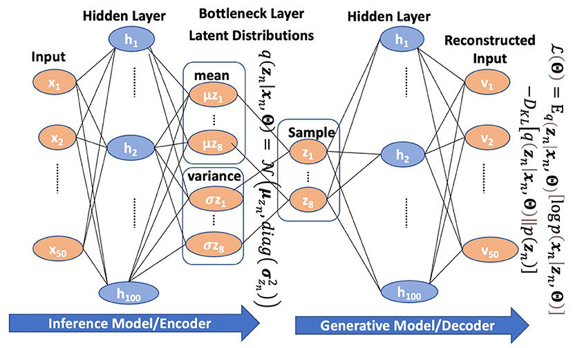
Figure 1. An example of a VAE with 100 hidden middle layer nodes and 8 bottleneck layer nodes.
The inference model estimates the posterior distribution of the latent factors in the bottleneck layer, which is assumed to be independent Gaussian. Consequently, the bottleneck layer consists of a vector of the means and a vector of the standard deviations of the posterior distribution. Then, samples drawn from the posterior distribution are passed to the generative model to reconstruct the original input data.
Input data represent an M × 1 vector of personality variable scores from sample n, and xmn denotes the mth personality variable. The xn is assumed to follow a multivariate independent Gaussian distribution, and its mean and variances are modeled as a function of an d-dimension latent representation of personality traits by an encoder neural network Dθ, where θ is a vector of encoder weights. Then the likelihood function of the input variable xn can be defined as
where Θ = {θ,ϕ} is the combined vector of encoder and decoder weights. Since xn only depends on the encoder weights, the model in (1) omitted decoder weights in the list of dependent variables. In VAE, zn is commonly assumed to follow a prior distribution, which is the multivariate standard normal, i.e., with Id being a d × d identity matrix.
The goal of training or inference is to compute the maximum likelihood estimate of Θ
where p(xn|Θ) = ∫p(xn|zn, Θ)p(zn)dzn is the marginal likelihood which is analytically intractable but can be lower bounded by the evidence lower bound (ELBO) L(Θ),
where q(zn|xn, Θ) is an approximate to the intractable posterior distribution p(zn|xn, Θ), and DKL[q(zn|xn, Θ) ||p(zn)] measures the Kullback-Leibler distance (Walters-Williams and Li, 2010) between the approximated posterior distribution q(zn|xn, Θ) and the prior distribution p(zn). To make the variational inference tractable, q(zn|xn, Θ) is assumed in most cases as a multivariate Gaussian,
whose means and variances are given by a decoder network Eϕ applied to xn as
where ϕ is the vector of the unknown decoder weights. Because of the approximation by in Equation (2) and the introduction of the decoder network in Equation (4), the model parameters to be estimated become Θ = {θ,ϕ}. Optimization of in Equation (2) is computed by the stochastic gradient descent algorithm, where the gradient is calculated by backpropagation. Note that the first part in Equation (3) will be proportional to the mean square error (MSE) between the input xn and the reconstructed scores vxn when we assume that the likelihood function of the personality variables follows an independent Gaussian distribution as in Equation (1). In VAE, the missing values are excluded when calculating the MSE.
VAE training is carried out with the TensorFlow machine learning module imported to Python (Jason, 2016).
Model Accuracy Metric and VAE Model Selection
We calculate the Person Correlation between the input personality variables and the reconstructed ones (input-reconstruction correlation) as the performance metric. The R2 statistics can be calculated sample-wise, i.e., between xn = [x1n, x2n, ⋯xMn] and vn = [v1n, v2n, ⋯vMn] n ∈ (1, N), or variable-wise, i.e. between for all variable indices m ∈ (1, M). Note that the reconstructed variables are assumed to be the sum of input variables plus independent noise after the input is put through an encoder and decoder function. Other commonly used performance measures in LFA, such as the communality or the percentage of variance represented by the selected factors, are not applicable in the context of VAE because these measures assume a linear data model between the factors and the input data, while the encoder and decoder in VAE are not linear.
In the context of LFA, to calculate the Person Correlation between the input and the reconstructed personality variable scores, we can first reconstruct the score for the mth personality variable in the nth sample, xmn based on the data model in LFA, which is a linear combination of d factors of the nth sample:
where is the vector of factor loadings in the mth personality variable, εm is the item specific factor, and σmn is the observation noise for the mth personality variable in the nth sample. Then the reconstructed score becomes vmn = if we assume that both εm and σmn have zero means. Then the correlation between the input and the reconstructed personality variables can be calculated either sample-wise or variable-wise for LFA.
The d latent factors are calculated both by the Thurstone and the Bartlett (Grice, 2001) methods. We compared the results of reconstruction and found that the two methods did not make a significant difference on input-reconstruction correlations in the tested datasets.
Note that in the machine learning community, the commonly used measure is Coefficient of Determinate (R2 statistics), which is defined as one minus the total error variance divided by the total sample variance. In the context of VAE, it can be viewed like communality in LFA, which measures how much variance has been explained.
In VAE, the mth personality variable's loadings on the ith factor, lmi, is estimated by calculating the correlation between the latent factor's mean vector , with the mth reconstructed input personality variable over all N training samples. Note that this loading is calculated for the purpose of finding a rotation of the factors such that the latent factors from different VAE runs can be aligned. We used the reconstructed inputs for loading calculation because the effect of noise has been removed after the reconstruction process and μzi represents the maximum posterior (MAP) estimation of the latent variables.
In LFA, the mth personality variable's loadings on the ith factor, lmi, is estimated by calculating the correlation between the vector of latent factor with the vector of the mth input personality variable over all N training samples. The calculation is performed by the factor analyzer in Python. Since we do not compare VAE and LFA in factor loadings, the difference in the calculation procedure of these loading factors is not consequential for the interpretation of the results.
VAE Factor Stability Analysis Based on Congruence Scores Over Multiple Runs
For LFA, noise factors beyond the first 5 did not appear consistently in different studies (Goldberg, 1990). Factors from different LFA runs could be rotated or perturbed due to variations, which can be attributed either to the analyzing methods or the datasets. Similarly, we also exclude noise factors and determine stable factors to be included in VAE constructed models.
The VAE employs a stochastic gradient descent algorithm that may not converge to the same solution across multiple runs. Such variations may introduce noise factors in addition to the ones introduced by the variations in the training datasets. To make sure that we only include stable factors in the final personality model, we extended the concept of congruence coefficient introduced by Goldberg for studying factor stability across different methods (Goldberg, 1990) and defined the congruence score between any two factors i and j in run r1 and run r2 as: , where represents the ith factor loadings on all M personality variables, and Corr() represents the Pearson correlation function.
In each VAE run, the latent factors are supposed to be independent and for each factor, only one factor from another run can be matched with it with a high congruence score. However, VAE often returns correlated factors within a run when we set the number of bottleneck layer nodes higher than the actual number of stable factors. In such cases, multiple factors from the same run may be clustered together with a given factor from another run. We observed that falsely matched factors generally have lower congruence scores than the true matching factors. To prevent the clustering algorithm from falsely matching factors, we set up a threshold and removed congruence scores below the threshold.
After the filtering step, the Leiden clustering algorithm (Traag et al., 2019) was applied to cluster factors from different runs. The Leiden clustering algorithm was developed to improve the Louvain algorithm. The Leiden algorithm allows both splitting and merging. The Leiden algorithm guarantees that clusters are well-connected and the clusters it finds are not too far from optimal.
All matching factors from all runs will be reported as clusters by the Leiden clustering algorithm. Then, we manually validated the clusters returned by the Leiden algorithm by inspecting the personality variables associated with each factor. To ensure that factors from different runs can be aligned together, we performed varimax rotation on the factor loadings before they were used to calculate the congruence scores.
To apply the clustering algorithm, d factor loading vectors from all R runs are retrieved for calculating a congruence score/factor loading correlation matrix with (dR) * (dR) elements. Then, the elements in the congruence score matrix below the threshold will be set to zero before it is fed into the Leiden clustering algorithms.
In practice, the threshold on the congruence scores was gradually raised until factors from the same run cannot be clustered together. We define a factor as stable when it can be identified in each VAE run. The average of the congruence scores within a cluster is used to represent the overall factor congruence.
We determine the final number of stable factors by increasing the number of bottleneck layer nodes until no more stable factors emerge.
Determining Factor-Variable Associations in VAE
After VAE identified a set of latent factors, it is important to understand how these factors can be interpreted. In LFA, this is done by inspecting the factor loadings of personality variables. However, since factor loadings are calculated by assuming a linear relationship between the factors and personality variables, we cannot apply the same method for identifying factor-variable association in VAE. We propose to inspect the reduction of correlations between the input and reconstructed personality variables. To calculate the reduction, we first set the investigated latent factor to zero, while the rest of the factors are fed into the VAE decoder to reconstruct the personality variables across all samples. Then, we calculate the correlations between the input and reconstructed variables after muting the investigated factor and compare it to the correlations before muting the factor. Personality variables with input-reconstruction correlation reduction above a threshold are associated with a latent factor. Since this method does not make any assumption on the linearity of the encoding and the decoding process, it is suitable for inspecting factor-variable association in both VAE and LFA.
Cross-Regional Study
To see whether the VAE returned factor model is valid across different regions, we trained a VAE model based on 80% of the samples from North America in the HEXACO analysis. Then, we estimated the factor statistics, especially the mean, the standard deviation, and the zero-order correlations of the derived factors to see if the factor model varies across different regions.
Linear Factor Analysis (LFA)
The LFA was conducted using the python function FactorAnalyzer imported from the sklearn.decomposition module (Persson and Khojasteh, 2021). Since previous research indicated that the selection of the LFA method would not make a significant difference in LFA (Goldberg, 1990), we used the principal factor method included in the package and selected ‘varimax' as the rotation method. The same scaled and normalized input data were used for both LFA and VAE.
Testing and Training Dataset Separation
We separated each input dataset into a training and a testing dataset by an 80–20% ratio. The training dataset was used for training the weights in the encoder and the decoder in VAE. It was also used to train the factor analyzer in LFA, which generated the factor loading matrix, a factor transformer (by default the Thurstone method) that can be used to calculate the factor scores, and other statistics, such as the eigenvalues of the data. We have also trained the weights for calculating the factor scores in the Bartlett method.
In VAE, the testing dataset was used to estimate the latent factors using the decoder, the reconstructed personality variables by using the encoder and the decoder, the input-reconstruction correlations, the congruence scores in factor stability analysis, and input-reconstruction correlation reduction in factor-variable association analysis. In LFA, the testing dataset was used to calculate the factor scores, the reconstructed personality variables, and the rest of the measures as in VAE.
In VAE training, the training dataset was further split into a training and validation dataset to ensure that the algorithm does not over-fit. The split ratio is 80–20%.
Complete separation between the training and the testing datasets is ensured. This procedure reduces the risk of overfitting because all testing was conducted on samples not included in the model construction process. Ten VAE models were trained using 10 training datasets in all analyses.
Results
Analysis of the IPIP Big 5 Dataset
LFA Exploratory Factor Analysis
We first conducted a LFA exploratory analysis by plotting the eigenvalues of the dataset. The scree plot in Figure 2 shows that there are 7 factors with eigenvalues greater than 1. If we look for the factors left to the elbow point, there are 5 factors in the data. Past research found that there are 5 stable factors (Costa and McCrae, 1992; Goldberg, 1992) that emerge from run to run. We can see that the results from the eigenvalue analysis and the scree plot are different and fewer factors can be generalized.
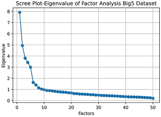
Figure 2. Exploratory factor analysis of the IPIP Big 5 dataset.
We then analyzed the factor-variable associations by inspecting the input-reconstruction correlation reduction as we increased the number of factors in LFA. An example result is shown in Figure 3 when there are 10 factors. We can see that the first 4 four factors of Extroversion, Neuroticism, Agreeableness, and Conscientiousness stayed the same as the original scale. However, the Openness factor fractionated in to 3 smaller factors, which makes the total number of factors to be 7.
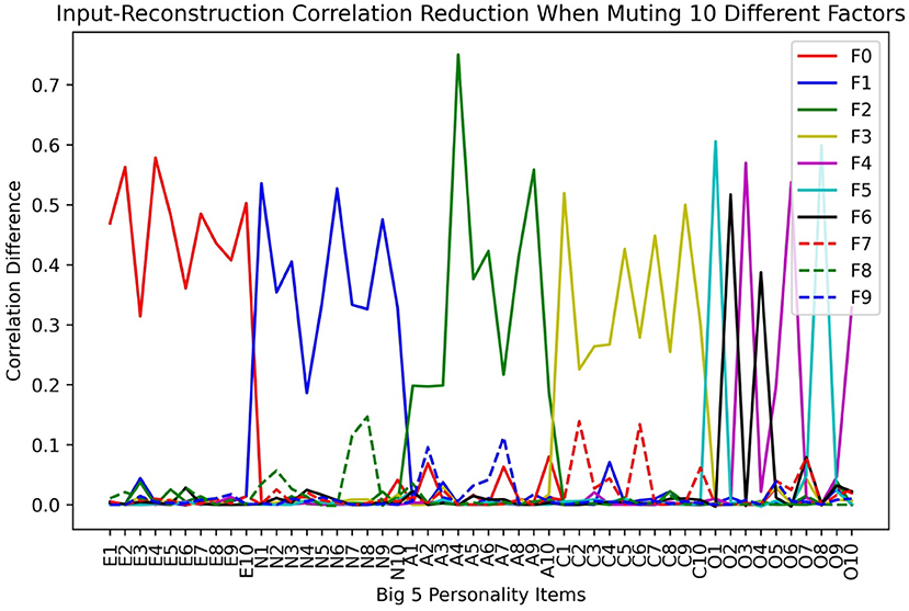
Figure 3. Input-reconstruction correlation reduction when assuming 10 Latent Factors in LFA.
VAE Analysis of the IPIP Big 5 Dataset
Model Parameter Selection
Model accuracy is measured by the variable-wise input-reconstruction correlations. Table 1 shows the results when using different numbers of hidden middle layers, different numbers of hidden middle layer nodes, and different numbers of bottleneck layer nodes. Note that the activation function of the last layer of the generative model is linear so that the output can have negative results. The activation function of bottleneck layer nodes must also be linear because they are assumed to be Gaussian variables. The Relu activation function was used for the rest of the layers.
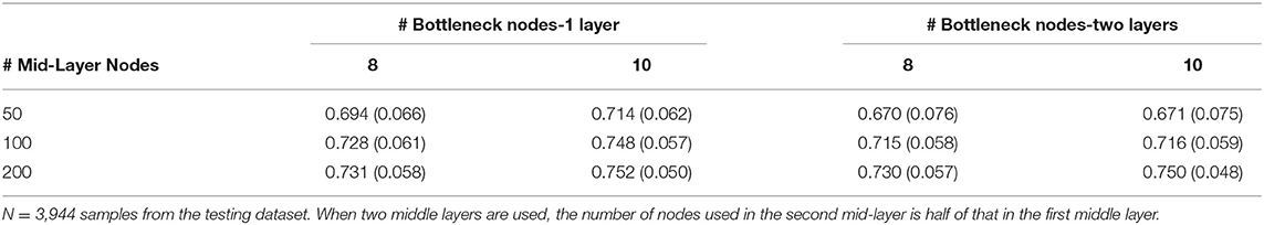
Table 1. The Mean (Std) of variable-wise input-reconstruction correlations.
Inspecting how the mean of the input-reconstruction correlations changes as we increase the number of middle layer nodes from 50 to 200 in Table 1, we can see that increasing the number of middle layer nodes constantly improves the performance, although increasing it beyond 100 nodes offered little performance gain. Further increasing the number of nodes does not change the factor structure or improve the correlations between the input and reconstructed variables significantly. Meanwhile the computational cost will grow significantly. Also, as the model becomes more complex, the required number of samples for appropriately estimating the weights in the deep neural network will increase. Another point is that in Table 1, it is evident that using two middle layers did not improve the performance. These observations hold with different the number of bottleneck layer nodes. Consequently, it should be sufficient to double the number of input layer nodes for the single middle layer.
To further investigate the impact of the number of bottleneck layer nodes, in Figure 4, we plot the means and the standard deviations of variable-wise input-reconstruction correlations. The number of latent factors was increased from 2 to 15. The standard deviations are indicated by the error bars in the plot. These results are evaluated based on the testing dataset with 3,944 samples.
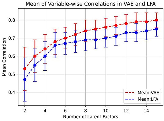
Figure 4. Mean of input-reconstruction correlations in VAE and LFA.
The improvement on the mean of correlations significantly slows down after the 5th latent factor in LFA, consistent with previous results (Costa and McCrae, 1992; Goldberg, 1992). On the other hand, the performance of VAE keeps on improving as the number of bottleneck layer nodes increases and there is not an obvious “elbow” point as in LFA for determining the number of factors to be extracted.
In Figure 5, we also compared R2 statistics in VAE to communality in LFA because it measures explained variance.
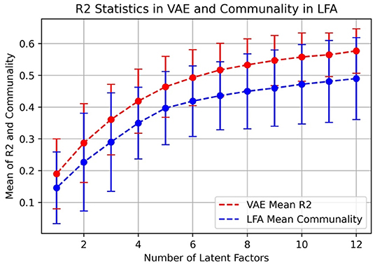
Figure 5. Mean of R2 statistics in VAE and communality in LFA.
We can see that in Figure 5, R2 statistics in VAE outperforms communality in LFA and the curves reflect the same trend as in Figure 4. Note that if the linear model in LFA completely holds, then communality should be the equivalent to R2. To plot (Figure 5), we first calculated the two measures (R2 and communality) for each variable, and then, we calculated the mean and standard deviation of the two measures across all 50 IPIP Big5 variables.
Factor Stability Analysis
From the plot in Figure 5, we cannot determine the number of factors that should be included in the personality model, and we further studied the stability of the discovered factors following the procedure outlined in the method section and summarized the results in Figure 6, in which we used 10 bottleneck layer nodes and 100 middle layer nodes.
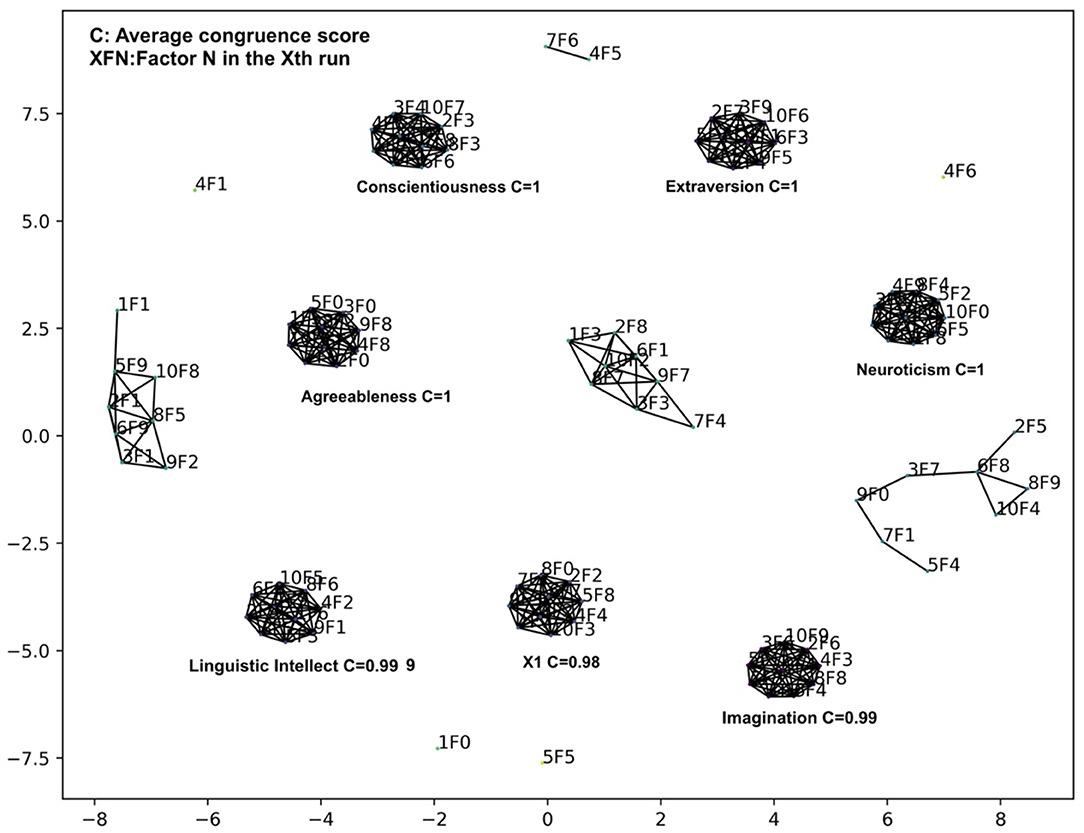
Figure 6. Clustering of factors from 10 VAE runs with 10 bottleneck layer nodes and 100 middle layer nodes in the Big 5 analysis.
After varimax rotation, we gradually raised the threshold on the congruence scores until no two factors from the same run could be clustered together. The threshold was set to 0.90. We can see that 7 stable factor clusters emerged with average congruence scores greater than 0.98. For the first 4 factors, Extraversion, Agreeableness, Conscientiousness, and Neuroticism, the top 10 personality variables ranked by factor loadings are the same as those in the original Big 5 model. The average congruence scores of these factor clusters are very high, which are rounded to one when two decimal points are considered. The rest of the 3 factors have a slightly smaller congruence score. Since factor loadings are not very appropriate for exploring factor-variable association in VAE and these factors have relatively less obvious interpretations, we temporarily mark them as Imagination, Linguistic Intellect, and a factor X1. The X1 did not have high loadings on any items and so we did not assign a name to it.
We also investigated the case of using 9 bottleneck layer nodes and 100 middle hidden layer nodes. The stability analysis results are included in Supplementary Figure 1.
Factor-Variable Associations
In Figure 7, we plot the input-reconstruction correlation reduction after muting each factor when 10 bottleneck layer nodes are used.
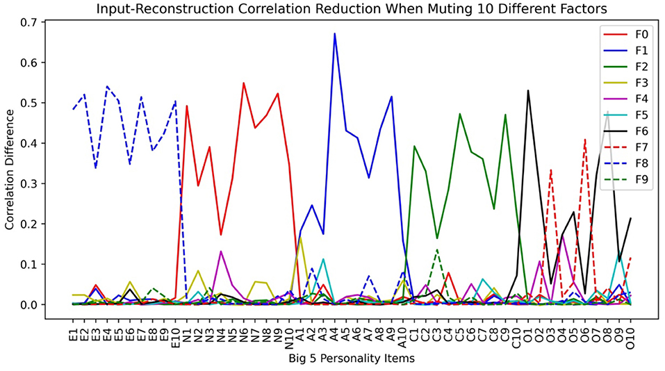
Figure 7. Input-reconstruction correlation reduction in a Big5 VAE run (E, Extraversion; N, Neuroticism; A, Agreeableness; C, Conscientiousness; O, Openness. See Table 2 for variable definitions).
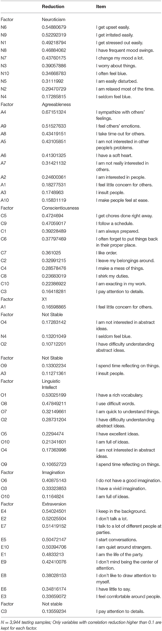
Table 2. Factor-variable association by inspecting input-reconstruction correlation reduction with 10 bottleneck layer nodes.
From Figure 7, we can see that the factor-variable associations are almost the same as in the LFA analysis. The openness factor fractionated into Imagination (F7 in Figure 7), Linguistic Intellect (F6), and X1 (F3). X1 is a minor factor in the sense that its main items have small reductions. However, it withstood the test of stability, and it cannot be ignored as noise. Compared to Figure 3, we can see that while LFA fractionated Openness into 3 factors, VAE fractionated it into two. LFA tends to fractionate more as we increase the number of assumed latent factors.
Inspecting the variables associated with each factor in Table 2, we can see that by using input-reconstruction correlation reduction, it is possible to identify factor-variable associations that mostly reproduce the results in the Big5 model.
We listed the correlations between the 7 factors in Table 3.
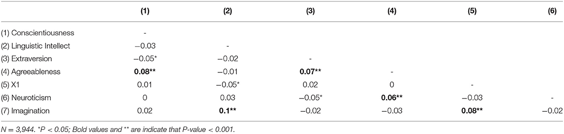
Table 3. Correlations between the 7 stable factors in the VAE IPIP Big 5 dataset analysis.
We have also calculated the sample-wise and variable-wise correlations between the reconstructed and the original inputs in both analyses over 3,944 testing samples and 50 personality variables. We used 7 hidden layer nodes for VAE and 7 factors for LFA for a fair comparison. We applied the Wilcoxon signed-rank test implemented in the SciPy package in python (Scipy Wilcoxon Signed-Rank Test Manual, n.d.) and calculated the p-values. The resulting statistics are shown in the box plots in Figure 8. They show that the 7-factor VAE model performs better than the 7-factor LFA model. The variance of variable-wise correlation is significantly smaller in VAE than LFA.
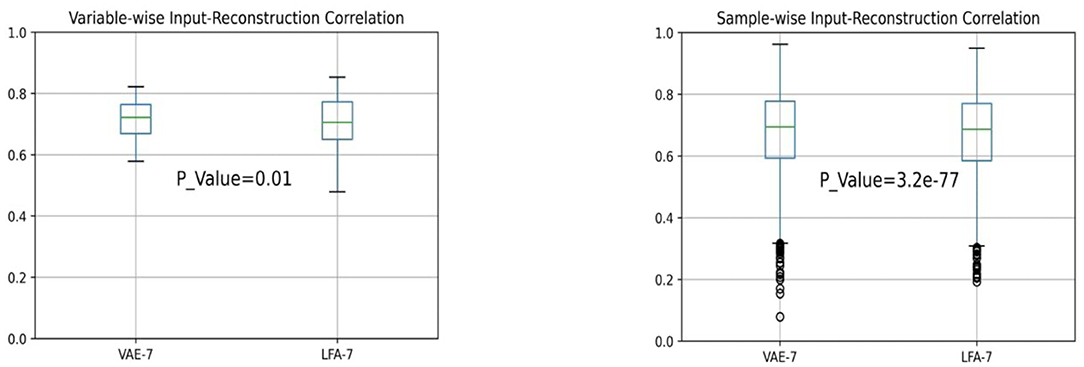
Figure 8. Variable-wise and sample-wise correlation statistics in VAE and LFA.
In this study, we can see that VAE mostly replicated the factor structure of the Big 5 scale initially discovered by LFA.
Analysis of the IPIP HEXACO Dataset
In the VAE analysis of the IPIP Big 5 data, the inventory only contains 50 personality variables. We wanted to investigate if VAE can be used when more personality variables are on the questionnaire and to verify if the factor selection principle derived in the first VAE analysis can be generalized. For this purpose, we applied VAE to an IPIP HEXACO dataset with 240 personality variables. We selected the model structure according to the principles derived previously. Also, since the IPIP HEXACO dataset has many more items than the Big5 dataset, we anticipated more factors.
LFA Analysis of the IPIP HEXACO Dataset
We first applied LFA analysis of the dataset and the resulting eigenvalues are plotted in the following scree plot:
From Figure 9, we can see that there are about 8 factors before the elbow point. However, if we applied the rule of selecting factors with eigenvalues greater than one, there are over 37 factors with eigenvalues above 1. Yet in the literature, the reported number of factors through LFA analysis is 6.
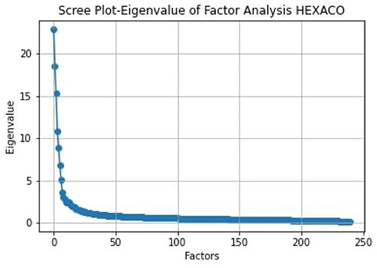
Figure 9. Scree plot of the eigenvalues in the HEXACO dataset.
Since there is a big discrepancy in the number of factors that should be extracted according to various factor extraction criteria, we investigated the factor structure when different numbers of latent factors are assumed in LFA. We first plotted the input-reconstruction correlation reduction plot when we assumed 6 latent factors and each of them was muted in turn in Figure 10. We can see that the plot reflects the standard HEXACO model structure because each factor is represented by a line with significant input-reconstruction correlation reduction over variables grouped for one factor and lower for other variables except some facets of Agreeableness and Humility-Honesty. Some of these facets are influenced by both the Agreeable and Humility-Honesty factor. We know that the factor level description is not sufficient to describe the complexity of the personality model. Personality variables associated with each factor are further divided into facets.
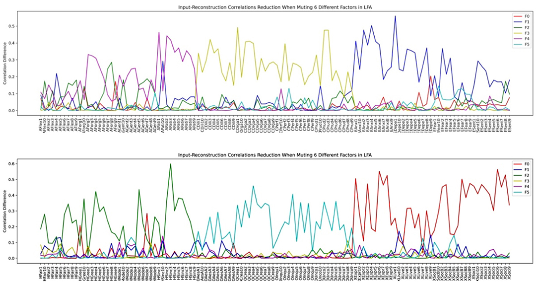
Figure 10. HEXACO factor- variable association when 6 latent factors are assumed in LFA (see section Methods for the list of acronyms).
We then investigated how the factor structure would change when we assume the number of latent factors to be 9 and 14 in Figures 11, 12, respectively.
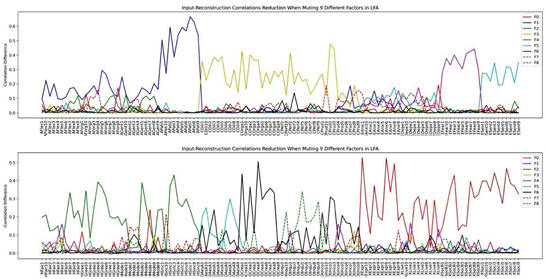
Figure 11. HEXACO factor-variable association when 9 latent factors are assumed in LFA.
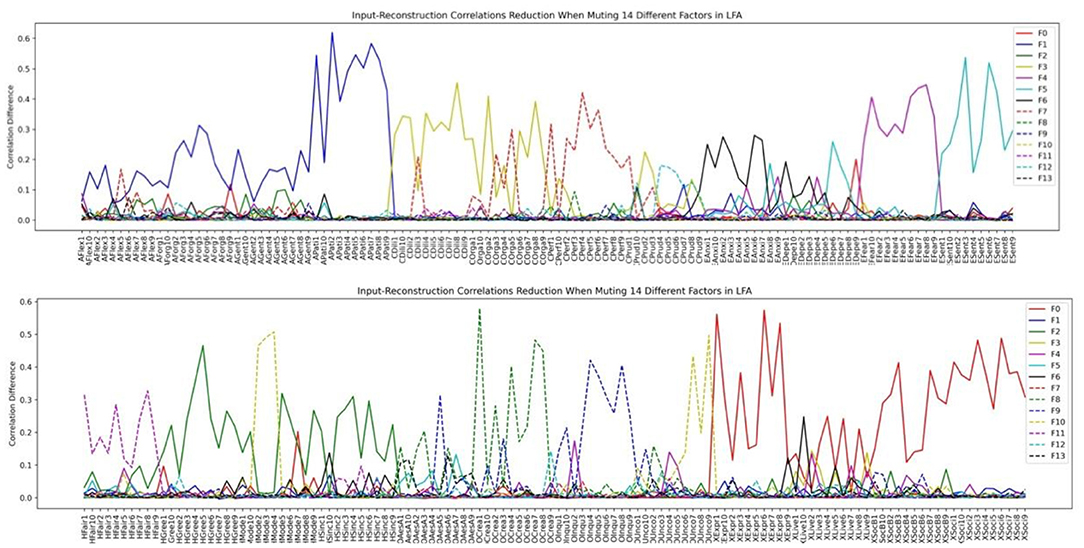
Figure 12. HEXACO factor-personality variable association when 14 latent factors are assumed in LFA.
Inspecting the factor structure when we assume 6, 9, and 14 factors, respectively, we can see that the factor structure keeps on fractionating without stability. The factor structure also does not improve the representation of the model as the number of factors increases. For example, the Depression and the Anxiety facet in Emotionality is well-represented in the 6-factor structure in Figure 10. However, when the number of factors is increased to 9, these two facets are influenced by several factors in which the factor plotted by the red dashed line (F7) is not representing any facet or factor (see the top half of Figure 11). In the case of 14 factors in Figure 12, we can see that except Extraversion and Agreeableness, all the rest of the factors are fractionated and there are 12 factors with a peak reduction greater than 0.2 and more than 5 variables. The structure is different from the 9-factor case, in which 9 factors have a peak reduction of greater than 0.2.
It is evident that when we apply LFA to factor analysis to a large set of personality variables, it is hard to determine the number of factors to be extracted based on eigenvalues or elbow points. The factor structure keeps on fractionating into smaller but still significant factors, and there is no definitive way to determine when to stop.
VAE Model Parameter Selection
We employed the model selection principles used in the VAE IPIP Big 5 dataset analysis. We set the number of nodes in the middle layer to 480, twice the number of input variables. Further increasing the number of nodes brought little improvement. A single middle layer between the input and the bottleneck layer was used and the activation function for the mid-layer was set to Relu. We gradually increased the number of bottleneck layer nodes to 12 and a maximum of 9 stable factors emerged in the analysis.
Factor Stability Analysis
The result of factor stability analysis on the 240 IPIP HEXACO variables is shown in Figure 13.
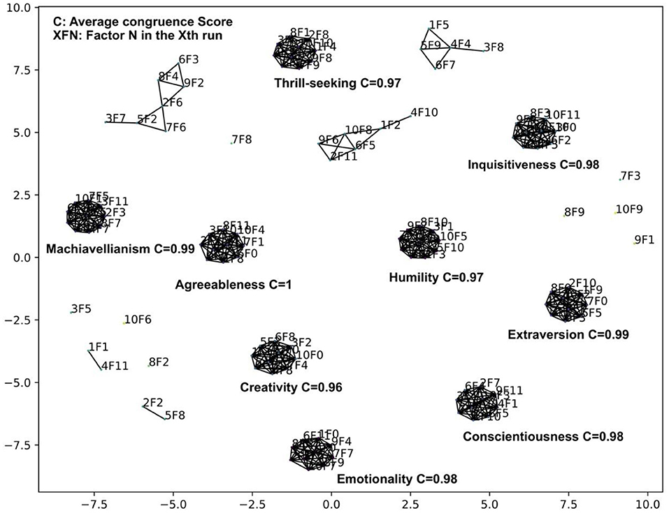
Figure 13. VAE analysis of the IPIP HEXACO dataset using 12 bottleneck layer nodes.
The filter threshold on the congruence scores was set to 0.875 such that no single factor is matched to two factors in another run. Nine stable factors with an average congruence score greater than 0.97 appeared across 10 VAE runs with 12 bottleneck layer nodes.
We then inspected the factor structure through the input-reconstruction correlation reduction plots when we set the number of bottleneck layer nodes to 9 and 14, respectively in Figures 14, 15.
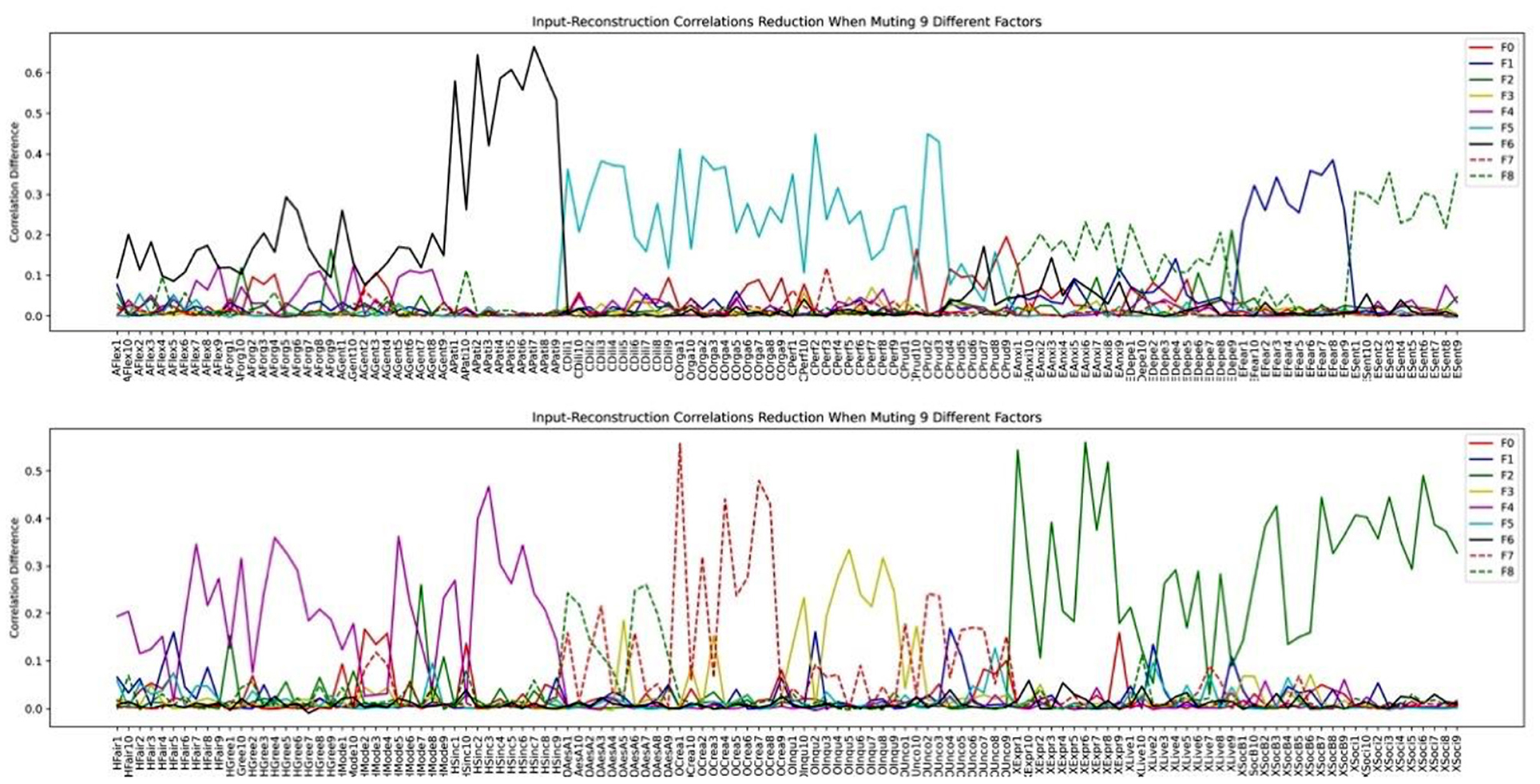
Figure 14. HEXACO factor-personality variable association when 9 latent factors are assumed in VAE.
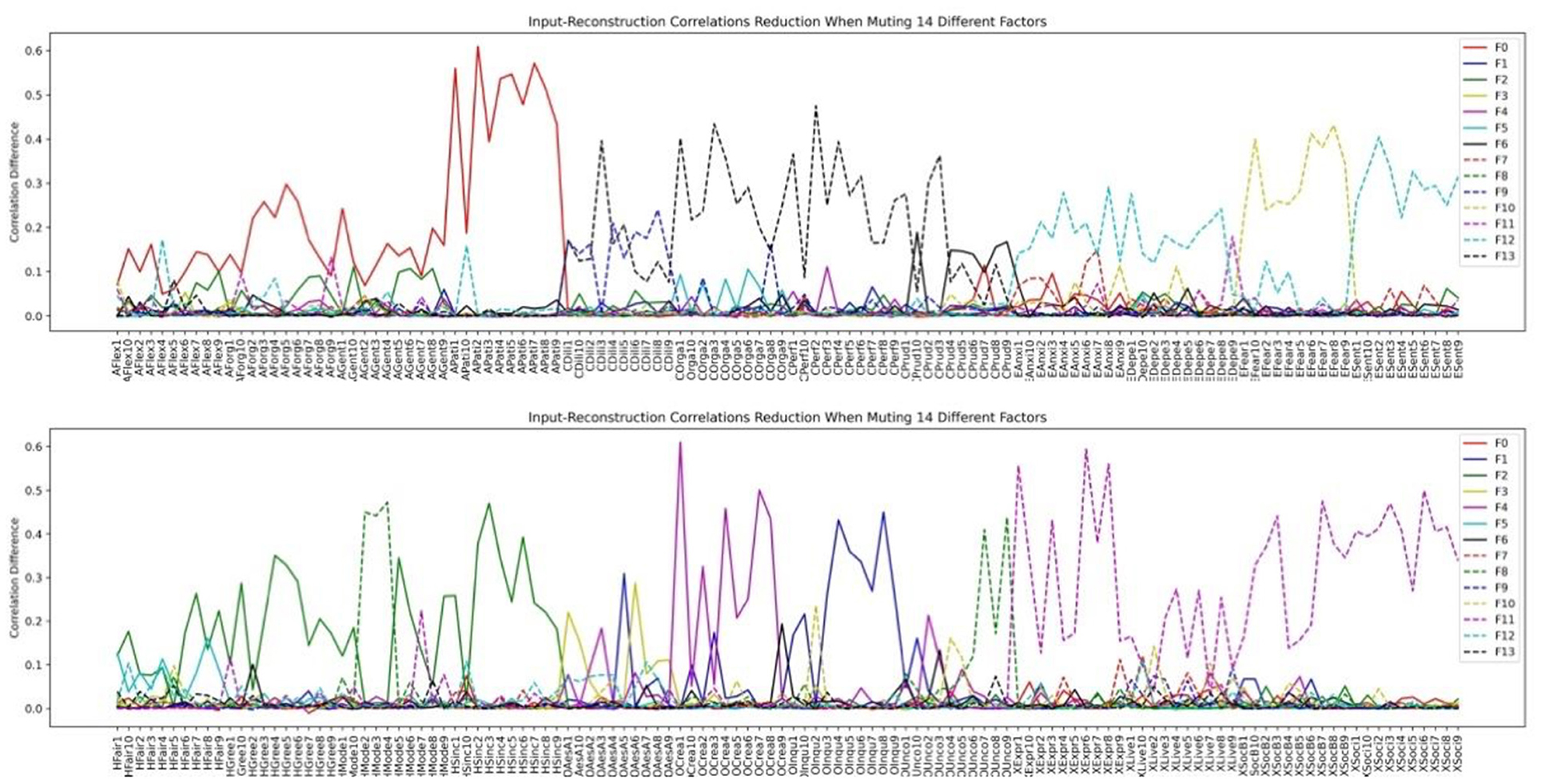
Figure 15. HEXACO factor-personality variable association when 14 latent factors are assumed in VAE.
Comparing Figures 14, 15, we can see that the factor structures are mostly the same. The top panel consists of 4 factors: Agreeableness, Conscientiousness, Thrill-seeking (the Fearfulness facet of Emotionality), Emotionality (All facets of Emotionality except the Fearfulness facet). The bottom panel consists of 4 major factors: Machiavellianism (All Humility-Honesty facets except two Modesty variables), Creativity (The Creativity facet of Openness to Experience), Inquisitiveness (The Inquisitiveness facet of Openness to Experience), and Extraversion. Humility (Two Modesty facet variables in Humility-Honesty plus several Unconventionality facet variables in Openness to Experience) appeared as a stable factor in both our VAE stability analysis and the 14-factor analysis (dashed green line in Figure 15).
Unlike the LFA analysis which keeps on fractionating as we increase the number of latent factors, VAE does not change the factor structure significantly and increasing the number of factors beyond the nine prominent factors added noise-like factors, such as F3, F5, F6, F7, F8 in Figure 15 (We define a factor as noise like factors when the maximum reduction on correlations is less than 0.1 and there are fewer than 5 items under the factor. Future research shall be conducted in terms of how to best chose these thresholds.). We can see that inspecting the limit on the number significant factors is a viable method for determining the number of factors to be extracted. We term this as the Significant Factor Limit Search (SFLS) method.
We conclude that by using VAE, we can determine the factor structure directly when a large pool of personality variables exists. Facet level analysis is not necessary since no significant factors can be discovered after the stable factors. Although we still cannot guarantee that the stability analysis or this SFLS method reports the true number of factors, at least in this case, the two types of analysis reported similar number of factors in HEXACO and Big 5. Unlike in LFA, the two types of analysis may return radically different number of factors especially when the set of analyzed personality variables are complex.
The zero-order correlations between the 9 discovered factors are listed in Table 4. The most significant correlations are highlighted in bold.
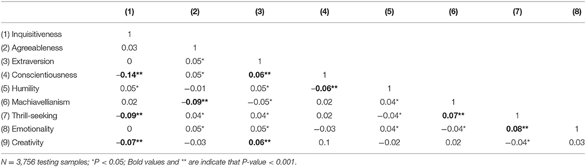
Table 4. Correlations between rotated factors in the IPIP HEXACO VAE analysis.
Cross-Regional Study
There is no significant deviation in mean, standard deviation. The mean and standard deviation statistics are included in the Supplementary Material. We further studied the zero-order correlations between the 9 factors in different regions. Again, little variation was detected. We listed the zero-order correlations in West Europe and Asia in Tables 5, 6 as examples. Please see the Supplementary Material for the rest of the regions.
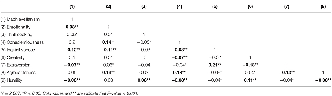
Table 5. Correlations between factors trained on North American samples and tested on West Europe samples.
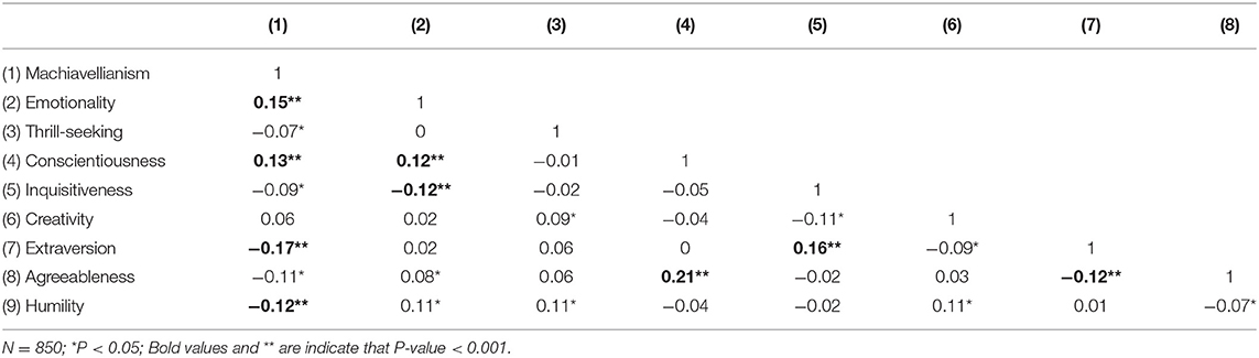
Table 6. Correlations between factors trained on North American samples and tested on Asian Samples.
Note that there are significantly larger correlations in the cross-regional study. This difference is caused by a smaller number of training samples, which affected the convergence of the VAE algorithm. The cross-region study was aimed at verifying the consistency of factor statistics across different regions, the results cannot be directly compared to the results obtained by using training samples from all regions.
Discussions
In this paper, we first investigated how VAE can be applied in exploring the factor structure in personality variables and how it compares to LFA. Past research showed that the personality model discovered via LFA must organize the scales at the factor and the facet level. When the number of investigated personality variables is large, LFA returns unstable factor structures as the number of assumed latent factors grows. LAF must cut a smaller number of factors such that the factors are generalizable. Yet, it is well-known that factor level representation alone is not sufficient and facet level information cannot be ignored when personality models are used for predicting various behaviors. In contrast, VAE returns stable factor structures even if the number of assumed latent factors is greater than the number of stable factors. Consequently, VAE can be applied to explore factor structures in a one-shot process given a pool of personality variables. A follow-up analysis at the facet level is not necessary and consequently, a lot of ad-hoc decisions can be avoided in the process.
This difference is due to VAE's inherent ability in dealing with non-linear data models. The fact that LFA cannot exhaust all useful information at the factor level is an indication of the non-linearity in the underlying personality model.
Note that VAE and LFA returned similar factor structures in the Big5 dataset. This shows that the 50 variables in the IPIP Big 5 dataset are mostly linearly related to the latent factors. On the other hand, the factor structures returned by VAE and LFA are very different in the more complicated HEXACO dataset, which indicates that the 240 variables in HEXACO are less linearly organized by the latent factors.
We aim to show that VAE is a viable analytical tool for exploratory factor analysis in this paper. The datasets we analyzed were collected using the IPIP Big 5 and IPIP HEXACO questionnaires for the purpose of comparison with LFA. We fully understand that the resulting factor models may not be comprehensive. There could still exist factors that the questionnaires have not covered, and self-reported data will limit the usefulness of the calculated model. Now, we will be able to extend the application of VAE to include various types of data in the future for constructing useful personality models.
For proper personality model development, VAE can be applied in a two-stage process: In stage one, the aim is to discover all essential and stable factors and select personality variables to represent all the factors properly. Comparing the stable factors found in the IPIP Big5 and the IPIP HEXACO analyses, we can see that similar factors can be discovered and aligned together even if the measured personality variables are not entirely identical. This suggests that in the future, we may perform a meta-analysis of multiple datasets and then pool all the discovered factors and their associated personality variables together for final analysis. In stage two, enough sample data should be collected for the pooled personality variables to construct a comprehensive personality model. Furthermore, it is anticipated that observer report data can be easily incorporated in the VAE framework as we can simply extend the input vector to include observer reported variables.
Limitations of VAE
The main limitation of effective VAE application is the number of samples available for analysis. For example, when we applied VAE on a reduced dataset with 2,099 samples, the reported mean (std) of the input-reconstruction correlations was 0.61 (0.08), which is significantly smaller than 0.65 (0.08) when all 18,779 samples are used in the HEXACO analysis. This indicates that VAE cannot converge to a lower cost function value without enough samples. VAE analysis requires a significantly larger number of samples than those required in LFA.
The required number of samples should also scale with the number of input variables. For example, in the IPIP HEXACO analysis, when we reduce the number of input variables to 79, the algorithm returns a much higher variable-wise mean correlation of 0.72 (0.08) than the case with 240 variables at 0.65 (0.08). However, if we reduce the number of input variables, some of the discovered factors will not be adequately represented by a group of personality variables just like the case of Big 5 dataset analysis. The pruning of the input items should be done carefully such that all factors are well represented.
We should balance the need to include more personality variables with the need to collect more samples, so that the VAE algorithm can converge properly. If the goal is to discover stable factors, then the average congruence score, the number of stable factors, and the reliability of the discovered factors can be used as guiding metrics in determining if enough samples have been included. One should evaluate if reducing the number of samples will affect the constructed model in all these statistics. If increasing the number of samples doesn't change the set of discovered stable factors, then the number of samples is enough.
If an accurate encoder is required, the guiding metric should be the mean and standard deviation of the input-reconstruction correlations. Enough samples should be included such that these measures can meet the requirement.
Another limitation of VAE is overfitting. To prevent this problem, besides a strict separation in the training testing dataset, we also monitor the loss function values calculated based on the training and the validation dataset. When the loss function value in the validation dataset does not decrease with the loss function in the training dataset, we stop the algorithm to prevent over-fitting.
While VAE-based factor analysis can be used to explore non-linear associations between latent factors and manifest personality variables, a common concern is the interpretability of the model. VAE does not have the equivalent measure of factor loading as in LFA. However, as we have demonstrated, the reduction of input-reconstruction correlations can be used as a substitute for examining factor-variable associations which returned similar results to that of factor loadings in LFA. Further research is needed to confirm its suitability as a measure for interpretating the discovered factors in VAE for practitioners to adopt it.
Future Research
In VAE, since we do not have a reliability measure as in LFA, we cannot determine what is adequate for representing a factor. In LFA, the convention in the field has been that each factor is represented by 5–10 variables with high alpha reliability. However, it seems that these calculated measures are never enough and a link to the biological basis is required for the factors to be called “adequate” in the view of some researchers. Ultimately, we should test how well VAE constructed factor structures can be used for various behavior predictions in comparison to LFA.
Another area for extending the current research is to incorporate observer report data into personality model construction. The hurdle lies in the availability of large observer datasets since it is much more difficult and costly to collect observer ratings. Nevertheless, given the increasing availability of various data and the complicated data structure, VAE shall find broad applications in such areas.
Data Availability Statement
The original contributions presented in the study are included in the article/Supplementary Material, further inquiries can be directed to the corresponding author/s. All code is made available on OSF (https://osf.io/6bf3w/).
Ethics Statement
Ethical review and approval was not required for the study on human participants in accordance with the local legislation and institutional requirements. Written informed consent from the patients/participants was not required to participate in this study in accordance with the national legislation and the institutional requirements.
Author Contributions
JZ came up with the idea of investigating personality model construction using deep learning methods, implemented the algorithm, and wrote the manuscript. YH identified variational autoencoder as the appropriate tool for the task and advised on the application of VAE to the problem. Both authors contributed to the article and approved the submitted version.
Conflict of Interest
The authors declare that the research was conducted in the absence of any commercial or financial relationships that could be construed as a potential conflict of interest.
Publisher's Note
All claims expressed in this article are solely those of the authors and do not necessarily represent those of their affiliated organizations, or those of the publisher, the editors and the reviewers. Any product that may be evaluated in this article, or claim that may be made by its manufacturer, is not guaranteed or endorsed by the publisher.
Acknowledgments
We thank reviewers for their helpful comments that have greatly improved the presentation of the paper.
Supplementary Material
The Supplementary Material for this article can be found online at: https://www.frontiersin.org/articles/10.3389/fpsyg.2022.863926/full#supplementary-material
References
Ahmad, H., Arif, A., Khattak, A. M., Habib, A., and Asghar, M. Z. (2020). “Applying deep neural networks for predicting dark triad personality trait of online users,” in 2020 International Conference on Information Networking (ICOIN), p. 102–5. IEEE. doi: 10.1109/ICOIN48656.2020.9016525
Ainsworth, S. K., Foti, N. J., and Lee, A. K. (2018). “Oi-VAE: output interpretable VAEs for nonlinear group factor analysis,” in International Conference on Machine Learning, p. 119–28. PMLR.
Ashton, M. C., and Lee, K. (2007). Empirical, theoretical, and practical advantages of the HEXACO model of personality structure. Personal. Soc. Psychol. Rev. 11, 150–166. doi: 10.1177/1088868306294907
Ashton, M. C., and Lee, K. (2008a). The HEXACO model of personality structure and the importance of the H factor. Soc. Personal. Psychol. Compass 2, 1952–1962. doi: 10.1111/j.1751-9004.2008.00134.x
Ashton, M. C., and Lee, K. (2008b). The prediction of honesty–humility-related criteria by the HEXACO and five-factor models of personality. J. Res. Personal. 42, 1216–1228. doi: 10.1016/j.jrp.2008.03.006
Ashton, M. C., Lee, K., and De Vries, R. E. (2014). The HEXACO honesty-humility, agreeableness, and emotionality factors: a review of research and theory. Personal. Soc. Psychol. Rev. 18, 139–152. doi: 10.1177/1088868314523838
Ashton, M. C., Lee, K., and Goldberg, L. R. (2007). The IPIP–HEXACO scales: an alternative, public-domain measure of the personality constructs in the HEXACO model. Personal. Indiv. Differ. 42, 1515–1526. doi: 10.1016/j.paid.2006.10.027
Avi, C., and Burshtein, D. (2020). Unsupervised Linear and Nonlinear Channel Equalization and Decoding Using Variational Autoencoders. IEEE Transac. Cogn. Commun. Netw. 6, 1003–1018. doi: 10.1109/TCCN.2020.2990773
Azucar, D., Marengo, D., and Settanni, M. (2018). Predicting the big 5 personality traits from digital footprints on social media: a meta-analysis. Personal. Indiv. Differ. 124, 150–59. doi: 10.1016/j.paid.2017.12.018
Baldi, P., and Hornik, K. (1989). Neural networks and principal component analysis: learning from examples without local minima. Neural Netw. 2, 53–58. doi: 10.1016/0893-6080(89)90014-2
Barrick, M. R., and Mount, M. K. (1991). The big five personality dimensions and job performance: a meta-analysis. Personnel Psychol. 44, 1–26. doi: 10.1111/j.1744-6570.1991.tb00688.x
Batmaz, Z., Yurekli, A., Bilge, A., and Kaleli, C. (2019). A review on deep learning for recommender systems: challenges and remedies. Artif. Intell. Rev. 52, 1–37. doi: 10.1007/s10462-018-9654-y
Baumeister, H., and Montag, C. (2019). Digital Phenotyping and Mobile Sensing. Basel: Springer International Publishing.
Bhavya, S., Pillai, A. S., and Guazzaroni, G. (2020). “Personality identification from social media using deep learning: a review,” in Soft Computing for Problem Solving. Singapore: Springer. p. 523–34. doi: 10.1007/978-981-15-0184-5_45
Bobadilla, J., Alonso, S., and Hernando, A. (2020). Deep learning architecture for collaborative filtering recommender systems. NATO Adv. Sci. Inst. Series E. 10, 2441. doi: 10.3390/app10072441
Bourlard, H., and Kamp, Y. (1988). Auto-association by multilayer perceptrons and singular value decomposition. Biol. Cyber. 59, 291–294. doi: 10.1007/BF00332918
Burgess, C. P., Higgins, I., Pal, A., Matthey, L., Watters, N., and Desjardins, G. (2018). Understanding disentangling in β-VAE. arXiv[Preprint].arXiv:1804.03599.
Carthy, A., Gray, G., McGuinness, C., and Owende, P. (2014). A review of psychometric data analysis and applications in modelling of academic achievement in tertiary education. J. Learn. Anal. 1, 57–106. doi: 10.18608/jla.2014.11.5
Castelvecchi, D. (2016). Deep learning boosts google translate tool. Nature. doi: 10.1038/nature.2016.20696
Cattell, R. B. (1943). The description of personality: basic traits resolved into clusters. J. Abnormal Soc. Psychol. 38, 476–506. doi: 10.1037/h0054116
Cattell, R. B., Eber, H. W., and Tatsuoka, M. M. (1970). Handbook for the Sixteen Personality Factor Questionnaire (16 PF): In Clinical, Educational, Industrial, and Research Psychology, for Use with All Forms of the Test. Institute for Personality and Ability Testing.
Chauhan, N. K., and Singh, K. (2018). “A review on conventional machine learning vs deep learning,” in 2018 International Conference on Computing, Power and Communication Technologies (GUCON). Greater Noida: IEEE. p. 347–52. doi: 10.1109/GUCON.2018.8675097
Chhabra, G. S., Sharma, A., and Krishnan, N. M. (2019). “Deep learning model for personality traits classification from text emphasis on data slicing,” in IOP Conference Series: Materials Science and Engineering. vol. 495, p. 012007. doi: 10.1088/1757-899X/495/1/012007
Costa, P. T., and McCrae, R. R. (1992). The five-factor model of personality and its relevance to personality disorders. J. Personality Diso. 6, 343–359. doi: 10.1521/pedi.1992.6.4.343
Cybenko, G. (1989). Approximation by Superpositions of a Sigmoidal Function. Mathem. Control, Sign. Syst. 2, 303–314. doi: 10.1007/BF02551274
De Vries, R. E., de Vries, A., and Feij, J. A. (2009). Sensation seeking, risk-taking, and the HEXACO model of personality. Personality Indiv. Differ. 47, 536–540. doi: 10.1016/j.paid.2009.05.029
Devlin, J., Chang, M. W., and Lee, K. (2018). BERT: pre-training of deep bidirectional transformers for language understanding. arXiv[Preprint].arXiv:1810.04805.
Eddine Bekhouche, S., Dornaika, F., and Ouafi, A. (2017). “Personality traits and job candidate screening via analyzing facial videos,” in Proceedings of the IEEE Conference on Computer Vision and Pattern Recognition Workshops (Honolulu, HI: IEEE), p. 10–13. doi: 10.1109/CVPRW.2017.211
Elngar, A. A., Jain, N., Sharma, D., Negi, H., and Trehan, A. (2020). A deep learning based analysis of the big five personality traits from handwriting samples using image processing. J. Inf. Technol. Manag. 12, 3–35. doi: 10.22059/JITM.2020.78884
Feher, A., and Vernon, P. A. (2021). Looking beyond the big five: a selective review of alternatives to the big five model of personality. Personal. Indiv. Differ. 169, 110002. doi: 10.1016/j.paid.2020.110002
Fiske, D. W. (1949). Consistency of the Factorial Structures of Personality Ratings from Different Sources. J. Abnormal Soc. Psychol. 44, 329–344. doi: 10.1037/h0057198
Goettfert, S., and Kriner, F., (n.d). Open-Source Psychometrics Project. Available online at: https://openpsychometrics.org/_rawdata (accessed August 10, 2021).
Goldberg, L. R. (1981). Language and individual differences: the search for universals in personality lexicons. Personal. Soc. Psychol. Rev. 2, 141–165.
Goldberg, L. R. (1990). An Alternative ‘Description of Personality': The Big-Five Factor Structure. J. Personality Soc. Psychol. 59, 1216–1229. doi: 10.1037/0022-3514.59.6.1216
Goldberg, L. R. (1992). The development of markers for the big-five factor structure. Psychol. Assess. 4, 26–42. doi: 10.1037/1040-3590.4.1.26
Goldberg, L. R. (1999). A broad-bandwidth, public domain, personality inventory measuring the lower-level facets of several five-factor models. Personal. Psychol. Europe. 7, 7–28.
Goldberg, L. R., and Saucier, G. (1998). What is beyond the big five? J. Personality. 66, 495–524. doi: 10.1111/1467-6494.00022
Grice, J. W. (2001). Computing and evaluating factor scores. Psychol. Method. 6, 430–450. doi: 10.1037/1082-989X.6.4.430
Hassan, H., Asad, S., and Hoshino, Y (2016). Determinants of leadership style in big five personality dimensions. Univ. J. Manage. 4, 161–179. doi: 10.13189/ujm.2016.040402
Higgins, I., Matthey, L., Pal, A., Burgess, C., Glorot, X., and Botvinick, M. (2016). Beta-VAE: learning basic visual concepts with a constrained variational framework. Available online at: https://openreview.net/pdf?id=Sy2fzU9gl (accessed December 20, 2013).
Horn, J. L. (1965). A rationale and test for the number of factors in factor analysis. Psychometrika 30, 179–85. doi: 10.1007/BF02289447
Hornik, K. (1991). Approximation capabilities of multilayer feedforward networks. Neural Net. 4, 251–257. doi: 10.1016/0893-6080(91)90009-T
Jacobson, K., Murali, V., Newett, E., and Whitman, B. (2016). “Music personalization at spotify,” in Proceedings of the 10th ACM Conference on Recommender Systems. RecSys '16. New York, NY, USA: Association for Computing Machinery. p. 373. doi: 10.1145/2959100.2959120
Jason, B. (2016). Deep Learning With Python: Develop Deep Learning Models on Theano and TensorFlow Using Keras. Machine Learning Mastery.
Jerram, K. L., and Coleman, P. G. (1999). The big five personality traits and reporting of health problems and health behaviour in old age. Br. J. Health Psychol. 4, 181–192. doi: 10.1348/135910799168560
Judge, T. A., and Bono, J. E. (2000). Five-factor model of personality and transformational leadership. J. Appl. Psychol. 85, 751–765. doi: 10.1037/0021-9010.85.5.751
Kim, J., Lee, J., and Park, E. (2020). A deep learning model for detecting mental illness from user content on social media. Sci. Rep. 10, 11846. doi: 10.1038/s41598-020-68764-y
Kingma, D. P., and Welling, M. (2013). Auto-encoding variational bayes. arXiv[Prepint].arXiv:1312.6114v.10..
Kingma, D. P., and Welling, M. (2019). An introduction to variational autoencoders. arXiv[Preprint].arXiv:1906.02691. doi: 10.1561/9781680836233
Krizhevsky, A., Sutskever, I., and Hinton, G. E. (2017). ImageNet classification with deep convolutional neural networks. Commun ACM. 60, 84–90. doi: 10.1145/3065386
Kumar, K. P., and Gavrilova, M. L. (2019). “Personality traits classification on Twitter,” in 2019 16th IEEE International Conference on Advanced Video and Signal Based Surveillance (AVSS), p. 1–8. doi: 10.1109/AVSS.2019.8909839
LeCun, Y., Bengio, Y., and Hinton, G. (2015). Deep learning. Nature 521, 436–444. doi: 10.1038/nature14539
Lee, K., and Ashton, M. C. (2004). Psychometric properties of the HEXACO personality inventory. Multiv. Behav. Res. 39, 329–358. doi: 10.1207/s15327906mbr3902_8
Lee, K., and Ashton, M. C. (2005). Psychopathy, machiavellianism, and narcissism in the five-factor model and the HEXACO model of personality structure. Personal. Indiv. Differ. 38, 1571–1582. doi: 10.1016/j.paid.2004.09.016
Liu, X., and Zhu, T. (2016). Deep learning for constructing microblog behavior representation to identify social media user's personality. PeerJ. Comput. Sci. 2, e81. doi: 10.7717/peerj-cs.81
Lopez-Alvis, J., Laloy, E., and Nguyen, F. (2020). Deep generative models in inversion: a review and development of a new approach based on a variational autoencoder. arXiv[Preprint].arXiv:2008.12056. doi: 10.1016/j.cageo.2021.104762
McCrae, R. R., Costa, P. T., Del Pilar, G. H., Rolland, J. P., and Parker, W. D. (1998). Cross-cultural assessment of the five-factor model: the revised NEO personality inventory. J. Cross-Cult. Psychol. 29, 171–188. doi: 10.1177/0022022198291009
Mehta, Y., Majumder, N., and Gelbukh, A. (2020). Recent trends in deep learning based personality detection. Artif. Intell. Rev. 53, 2313–2339. doi: 10.1007/s10462-019-09770-z
Noftle, E. E., and Robins, R. W. (2007). Personality predictors of academic outcomes: big five correlates of GPA and SAT scores. J. Personality Soc. Psychol. 93, 116–130. doi: 10.1037/0022-3514.93.1.116
Norman, W. T. (1963). Toward an adequate taxonomy of personality attributes: replicated factor structure in peer nomination personality ratings. J. Abnormal Soc. Psychol. doi: 10.1037/h0040291
O'Meara, M. S., and South, S. C. (2019). Big five personality domains and relationship satisfaction: direct effects and correlated change over time. J. Personality 87, 1206–1220. doi: 10.1111/jopy.12468
Persson, I., and Khojasteh, J. (2021). Python packages for exploratory factor analysis. Struct. Equat. Model. 28, 983–8. doi: 10.1080/10705511.2021.1910037
Remaida, A., Moumen, A., and El Idrissi, Y. E. B. (2020). “Handwriting personality recognition with machine learning: a comparative study,” in: 2020 IEEE 2nd International Conference on Electronics, Control, Optimization and Computer Science (ICECOCS), p. 1–6. Kenitra: IEEE. doi: 10.1109/ICECOCS50124.2020.9314529
Ren, Z., Shen, Q., and Diao, X. (2021). A sentiment-aware deep learning approach for personality detection from text. Inf. Process. Manage. 58, 102532. doi: 10.1016/j.ipm.2021.102532
Reynolds, S. K., and Clark, L. A. (2001). Predicting dimensions of personality disorder from domains and facets of the five-factor model. J. Personal. 69, 199–222. doi: 10.1111/1467-6494.00142
Rodriguez, P., Gonzàlez, J., and Gonfaus, J. M. (2019). Integrating vision and language in social networks for identifying visual patterns of personality traits. Int. J. Soc. Sci. Humanit. 9, 6–12. doi: 10.18178/ijssh.2019.V9.981
Salminen, J., Rao, R. G., Jung, S. G., Chowdhury, S. A., and Jansen, B. J. (2020). “Enriching social media personas with personality traits: a deep learning approach using the big five classes,” in Artificial Intelligence in HCI. Springer International Publishing. p. 101–20. doi: 10.1007/978-3-030-50334-5_7
Samuel, D. B., and Widiger, T. A. (2008). A meta-analytic review of the relationships between the five-factor model and DSM-IV-TR personality disorders: a facet level analysis. Clin. Psychol. Rev. 28, 1326–1342. doi: 10.1016/j.cpr.2008.07.002
Saulsman, L. M., and Page, A. C. (2004). The five-factor model and personality disorder empirical literature: a meta-analytic review. Clin. Psychol. Rev. 23, 1055–1085. doi: 10.1016/j.cpr.2002.09.001
Scipy Wilcoxon Signed-Rank Test Manual. (n.d.). Available online at: https://docs.scipy.org/doc/scipy/reference/generated/scipy.stats.wilcoxon.html (accessed November 10, 2021).
Sengupta, S., Basak, S., Saikia, P., Paul, S., Tsalavoutis, V., Atiah, F., et al. (2020). A review of deep learning with special emphasis on architectures, applications and recent trends. Knowl. Based Syst. 194, 105596. doi: 10.1016/j.knosys.2020.105596
Spathis, D., Servia-Rodriguez, S., Farrahi, K., and Mascolo, C. (2019). “Passive mobile sensing and psychological traits for large scale mood prediction,” in Proceedings of the 13th EAI International Conference on Pervasive Computing Technologies for Healthcare. PervasiveHealth'19. New York, NY, USA: Association for Computing Machinery. p. 272–81. doi: 10.1145/3329189.3329213
Sun, P., Kretzschmar, H., Dotiwalla, X., Chouard, A., Patnaik, V., and Tsui, P. (2020). “Scalability in perception for autonomous driving: waymo open dataset,” in Proceedings of the IEEE/CVF Conference on Computer Vision and Pattern Recognition (IEEE), p. 2446–54. doi: 10.1109/CVPR42600.2020.00252
Tan, Q., Gao, L., Lai, Y. K., and Xia, S. (2018). “Variational autoencoders for deforming 3d mesh models,” in Proceedings of the IEEE Conference on Computer Vision and Pattern Recognition (Salt Lake City, UT: IEEE), p. 5841–50. doi: 10.1109/CVPR.2018.00612
Traag, V. A., Waltman, L., and Van Eck, N. J. (2019). From Louvain to Leiden: guaranteeing well-connected communities. Sci. Rep. 9, 5233. doi: 10.1038/s41598-019-41695-z
Tupes, E. C., and Christal, R. E. (1961). Recurrent personality factors based on trait ratings. J. Personal. 60, 225–251. doi: 10.1111/j.1467-6494.1992.tb00973.x
Urban, C. J., and Bauer, D. J. (2021). A deep learning algorithm for high-dimensional exploratory item factor analysis. Psychometrika 86, 1–29. doi: 10.1007/s11336-021-09748-3
Walters-Williams, J., and Li, Y. (2010). “Comparative study of distance functions for nearest neighbors,” in Advanced Techniques in Computing Sciences and Software Engineering. Netherlands: Springer. p. 79–84. doi: 10.1007/978-90-481-3660-5_14
Wang, K., Forbes, M. G., Gopaluni, B., Chen, J., and Song, Z. (2019). Systematic development of a new variational autoencoder model based on uncertain data for monitoring nonlinear processes. IEEE Access. 7, 22554–22565. doi: 10.1109/ACCESS.2019.2894764
Widiger, T. A., and Lowe, J. R. (2007). Five-factor model assessment of personality disorder. J. Personality Assessm. 89, 16–29. doi: 10.1080/00223890701356953
Yu, J., and Markov, K. (2017). “Deep learning based personality recognition from facebook status updates,” in 2017 IEEE 8th International Conference on Awareness Science and Technology (iCAST). Taichung: IEEE. p. 383–87. doi: 10.1109/ICAwST.2017.8256484
Zemel, R. S., and Hinton, G. E. (1993). “Developing population codes for object instantiation parameters,” in AAAI Fall Symposium Series: Machine Learning in Computer Vision Raleigh. North Carolina USA. Available online at: https://www.aaai.org/Papers/Symposia/Fall/1993/FS-93-04/FS93-04-022.pdf (accessed December 20, 2013).
Zhou, D., and Wei, X. X. (2020). Learning identifiable and interpretable latent models of high-dimensional neural activity using Pi-VAE. Adv. Neural Inf. Process. Syst. 33, 7234–7247.
Keywords: non-linear factor analysis, variational auto encoder (VAE), personality trait, artificial intelligence, Big 5 personality factors, HEXACO model of personality, deep learning
Citation: Huang Y and Zhang J (2022) Exploring Factor Structures Using Variational Autoencoder in Personality Research. Front. Psychol. 13:863926. doi: 10.3389/fpsyg.2022.863926
Received: 14 February 2022; Accepted: 07 April 2022;
Published: 05 August 2022.
Edited by:
Alexander Robitzsch, IPN - Leibniz Institute for Science and Mathematics Education, GermanyReviewed by:
David Goretzko, Ludwig Maximilian University of Munich, GermanyAndrew Cutler, Boston University, United States
Steffen Nestler, University of Münster, Germany
Copyright © 2022 Huang and Zhang. This is an open-access article distributed under the terms of the Creative Commons Attribution License (CC BY). The use, distribution or reproduction in other forums is permitted, provided the original author(s) and the copyright owner(s) are credited and that the original publication in this journal is cited, in accordance with accepted academic practice. No use, distribution or reproduction is permitted which does not comply with these terms.
*Correspondence: Jianqiu Zhang, bWljaGVsbGUuemhhbmdAdXRzYS5lZHU=