Scrutinizing GW-Based Methods Using the Hubbard Dimer

Using the simple (symmetric) Hubbard dimer, we analyze some important features of the GW approximation. We show that the problem of the existence of multiple quasiparticle solutions in the (perturbative) one-shot GW method and its partially self-consistent version is solved by full self-consistency. We also analyze the neutral excitation spectrum using the Bethe-Salpeter equation (BSE) formalism within the standard GW approximation and find, in particular, that 1) some neutral excitation energies become complex when the electron-electron interaction U increases, which can be traced back to the approximate nature of the GW quasiparticle energies; 2) the BSE formalism yields accurate correlation energies over a wide range of U when the trace (or plasmon) formula is employed; 3) the trace formula is sensitive to the occurrence of complex excitation energies (especially singlet), while the expression obtained from the adiabatic-connection fluctuation-dissipation theorem (ACFDT) is more stable (yet less accurate); 4) the trace formula has the correct behavior for weak (i.e., small U) interaction, unlike the ACFDT expression.

1 Introduction

Many-body perturbation theory (MBPT) based on Green’s functions is among the standard tools in condensed matter physics for the study of ground- and excited-state properties. (Aryasetiawan and Gunnarsson, 1998; Onida et al., 2002; Martin et al., 2016; Golze et al., 2019). In particular, the GW approximation (Hedin, 1965; Golze et al., 2019) has become the method of choice for band-structure and photoemission calculations and, combined with the Bethe-Salpeter equation (BSE@GW) formalism, (Salpeter and Bethe, 1951; Strinati, 1988; Albrecht et al., 1998; Rohlfing and Louie, 1998; Benedict et al., 1998; van der Horst et al., 1999a; Blase et al., 2018, 2020), for optical spectra calculations. Thanks to efficient implementations, (Duchemin and Blase, 2019, 2020, 2021; Bruneval et al., 2016; van Setten et al., 2013; Kaplan et al., 2015, 2016; Krause and Klopper, 2017; Caruso et al., 2012, 2013b,a; Caruso, 2013; Wilhelm et al., 2018), this toolkit is acquiring increasing popularity in the traditional quantum chemistry community, (Rohlfing and Louie, 1999; van der Horst et al., 1999b; Puschnig and Ambrosch-Draxl, 2002; Tiago et al., 2003; Boulanger et al., 2014; Jacquemin et al., 2015b; Bruneval et al., 2015; Jacquemin et al., 2015a; Hirose et al., 2015; Jacquemin et al., 2017a,b; Rangel et al., 2017; Krause and Klopper, 2017; Gui et al., 2018; Blase et al., 2018; Liu et al., 2020; Blase et al., 2020; Holzer and Klopper, 2018; Holzer et al., 2018; Loos et al., 2020), partially due to the similarity of the equation structure to that of the standard Hartree-Fock (HF) (Szabo and Ostlund, 1989) or Kohn-Sham (KS) (Hohenberg and Kohn, 1964; Kohn and Sham, 1965) mean-field methods. Several studies of the performance of various flavors of GW in atomic and molecular systems are now present in the literature, (Holm and von Barth, 1998; Stan et al., 2006; Stan et al., 2009; Blase and Attaccalite, 2011; Faber et al., 2011; Bruneval, 2012; Bruneval and Marques, 2013; Bruneval et al., 2015; Karlsson and van Leeuwen, 2016; Bruneval et al., 2016; Bruneval, 2016; Boulanger et al., 2014; Blase et al., 2016; Li et al., 2017; Hung et al., 2016, 2017; van Setten et al., 2015, 2018; Ou and Subotnik, 2016, 2018; Faber, 2014), providing a clearer picture of the pros and cons of this approach. There are, however, still some open issues, such as 1) how to overcome the problem of multiple quasiparticle solutions, (van Setten et al., 2015; Maggio et al., 2017; Loos et al., 2018; Véril et al., 2018; Duchemin and Blase, 2020; Loos et al., 2020), 2) what is the best way to calculate ground-state total energies, (Casida, 2005; Huix-Rotllant et al., 2011; Caruso et al., 2013b; Casida and Huix-Rotllant, 2016; Colonna et al., 2014; Olsen and Thygesen, 2014; Hellgren et al., 2015; Holzer et al., 2018; Li et al., 2019, 2020; Loos et al., 2020), and 3) what are the limits of the BSE in the simplification commonly used in the so-called Casida equations. (Strinati, 1988; Rohlfing and Louie, 2000; Sottile et al., 2003; Myöhänen et al., 2008; Ma et al., 2009a,b; Romaniello et al., 2009b; Sangalli et al., 2011; Huix-Rotllant et al., 2011; Sakkinen et al., 2012; Zhang et al., 2013; Rebolini and Toulouse, 2016; Olevano et al., 2019; Lettmann and Rohlfing, 2019; Loos and Blase, 2020; Authier and Loos, 2020; Monino and Loos, 2021). In the present work, we address precisely these questions by using a very simple and exactly solvable model, the symmetric Hubbard dimer. Small Hubbard clusters are widely used test systems for the GW approximation (e.g. Verdozzi et al., 1995; Schindlmayr et al., 1998; Pollehn et al., 1998; Puig von Friesen et al., 2010; Romaniello et al., 2009a, 2012). Despite its simplicity, the Hubbard dimer is able to capture lots of the underlying physics observed in more realistic systems, (Romaniello et al., 2009a, 2012; Carrascal et al., 2015, 2018), such as, for example, the nature of the band-gap opening in strongly correlated systems as bulk NiO. (Di Sabatino et al., 2016). Here, we will use it to better understand some features of the GW approximation and the BSE@GW approach. Of course, care must be taken when extrapolating conclusions to realistic systems.

The paper is organized as follows. Section 2 provides the key equations employed in MBPT to calculate removal and addition energies (or charged excitations), neutral (or optical) excitation energies, and ground-state correlation energies. In Sec. 3, we present and discuss the results that we have obtained for the Hubbard dimer. We finally draw conclusions and perspectives in Sec. 4.

2 Theoretical Framework

In the following we provide the key equations of MBPT (Martin et al., 2016) and, in particular, we discuss how one can calculate ground- and excited-state properties, namely removal and addition energies, spectral function, total energies, and neutral excitation energies. We use atomic units ℏ = m = e = 1 and work at zero temperature throughout the paper.

2.1 The GW Approximation

Within MBPT a prominent role is played by the one-body Green’s function G which has the following spectral representation in the frequency domain:

$G({\mathit{x}}_1,{\mathit{x}}_2;\omega )=\sum _{\nu }\frac{{\psi }_{\nu }({\mathit{x}}_1){\psi }_{\nu }^{*}({\mathit{x}}_2)}{\omega -{ϵ}_{\nu }+\text{i}\eta \text{sgn}({ϵ}_{\nu }-\mu )},(1)$

where μ is the chemical potential, η is a positive infinitesimal, ${ϵ}_{\nu }=E_{\nu }^{N+1}-E_0^N$ for ε_ν > μ, and ${ϵ}_{\nu }=E_0^N-E_i^{N-1}$ for ε_ν < μ. Here, $E_{\nu }^N$ is the total energy of the νth excited state of the N-electron system (ν = 0 being the ground state). In the case of single-determinant many-body wave functions (such as HF or KS), the so-called Lehmann amplitudes ψ_ν (x) reduce to one-body orbitals and the poles of the Green’s function ε_ν to one-body orbital energies.

The one-body Green’s function is a powerful quantity that contains a wealth of information about the physical system. In particular, as readily seen from Eq. 1, it has poles at the charged excitation energies of the system, which are proper addition/removal energies of the N-electron system. Thus, one can also access the (photoemission) fundamental gap

$E_{\text{g}}=I^N-A^N,(2)$

where $I^N=E_0^{N-1}-E_0^N$ is the ionization potential and $A^N=E_0^N-E_0^{N+1}$ is the electron affinity. Moreover, one can straightforwardly obtain the spectral function, which is closely related to photoemission spectra, as

$A({\mathit{x}}_1,{\mathit{x}}_2;\omega )=\frac{1}{\pi }\text{sgn}(\mu -\omega )\mathrm{Im}G({\mathit{x}}_1,{\mathit{x}}_2;\omega ).(3)$

The ground-state total energy can also be extracted from G using the Galitskii-Migdal (GM) formula (Galitskii and Migdal, 1958)

$E_0^{\text{GM}}=-\frac{\text{i}}{2}\int {d\mathit{x}}_1\underset{2\to 1^{+}}{\lim }\left[\text{i}\frac{\partial }{\partial t_1}+h({\mathit{r}}_1)\right]G(\mathrm{1,2}),(4)$

where 1 ≡ (x₁, t₁) is a space-spin plus time composite variable and h(r) = − ∇/2 + v_ext(r) is the one-body Hamiltonian, v_ext (r) being the local external potential.

The one-body Green’s function can be obtained by solving a Dyson equation of the form G = G₀ + G₀ΣG, where G₀ is the non-interacting Green’s function and the self-energy Σ is an effective potential which contains all the many-body effects of the system under study. In practice, Σ must be approximated and a well-known approximation is the so-called GW approximation in which the self-energy reads Σ^GW = v_H + iGW, where v_H is the classical Hartree potential, and W = ɛ⁻¹v_c is the dynamically screened Coulomb interaction, with ɛ⁻¹ the inverse dielectric function and v_c the bare Coulomb interaction. (Hedin, 1965).

The equations stemming from the GW approximation should, in principle, be solved self-consistently, since Σ is a functional of G. (Hedin, 1965). Self-consistency, however, is computationally demanding, and one often performs a single GW correction (for example using G₀ as starting point one builds W and Σ^GW as Σ^GW = v_H + iG₀W₀, with v_H = − iv_cG₀ and $W_0={[1+\text{i}{v}_c{G}_0{G}_0]}^{-1}{v}_c$, from which $G={\{1-G_0{\mathrm{\Sigma }}^{GW}[G_0]\}}^{-1}{G}_0$). This cost-saving and popular strategy is known as one-shot GW. The main drawback of the one-shot GW method is its dependence on the starting point (i.e., the orbitals and energies of the HF or KS mean-field eigenstates) originating from its perturbative nature. To overcome this problem, one can introduce some level of self-consistency. Removal/addition energies are thus obtained by solving iteratively the so-called quasiparticle equation

$\omega ={ϵ}_i^{\text{HF}}+\left.⟨{\varphi }_i^{\text{HF}}\right|{\mathrm{\Sigma }}_{\text{c}}^{GW}(\omega )\left|{\varphi }_i^{\text{HF}}\right.⟩.(5)$

Here, we choose to start from HF spatial orbitals ${\varphi }_i^{\text{HF}}(\mathit{r})$ and energies ${ϵ}_i^{\text{HF}}$, which are corrected by the (real part of the) correlation contribution of the GW self-energy ${\mathrm{\Sigma }}_{\text{c}}^{GW}={\mathrm{\Sigma }}^{GW}-{\mathrm{\Sigma }}_{\text{HF}}$, where Σ_HF = v_H + iv_cG is the HF (hartree plus exchange) contribution to the self-energy. ${\mathrm{\Sigma }}_c^{GW}$ is evaluated with G_HF at the first iteration, where G_HF is the self-consistent solution of G_HF = G₀ + G₀Σ^HFG_HF. At the nth iteration, ${\mathrm{\Sigma }}_c^{GW}$ is evaluated as ${\mathrm{\Sigma }}_c^{GW}[G^{n-1}]$, where Gⁿ⁻¹ has poles at the energies from the (n − 1)-th iteration of Eq. 5 and corresponding weights obtained from the Z factors given in Eq. 6. As a non-linear equation, Eq. 5 has potentially many solutions ${ϵ}_{i,\nu }^{GW}$. The so-called quasiparticle (QP) solution ${ϵ}_{i,\nu =0}^{GW}\equiv {ϵ}_i^{\text{QP}}$ has the largest renormalization factor (or spectral intensity)

$Z_{i,\nu }={\left[1-{\left.\left.⟨{\varphi }_i^{\text{HF}}\right|\frac{\partial {\mathrm{\Sigma }}_{\text{c}}^{GW}(\omega )}{\partial \omega }\left|{\varphi }_i^{\text{HF}}\right.⟩\right|}_{\omega ={ϵ}_{i,\nu }^{GW}}\right]}^{-1},(6)$

while the satellite (sat) peaks ${ϵ}_{i,\nu >0}^{GW}\equiv {ϵ}_{i,\nu }^{\text{sat}}$ share the remaining of the spectral weight. Moreover, one can show that the following sum rule is fulfilled (von Barth and Holm, 1996)

$\sum _{\nu }{Z}_{i,\nu }=1,(7)$

where the sum runs over all the solutions of the quasiparticle equation for a given mean-field eigenstate i. Throughout this article, i, j, k, and l denote general spatial orbitals, a and b refer to occupied orbitals, r and s to unoccupied orbitals, while m labels single excitations a → r.

In eigenvalue self-consistent GW (commonly abbreviated as evGW), (Hybertsen and Louie, 1986; Shishkin and Kresse, 2007; Blase and Attaccalite, 2011; Faber et al., 2011; Rangel et al., 2016; Gui et al., 2018), one only updates the poles of G, while keeping fix the orbitals (or weights). G is then used to build Σ^GW and W. At the nth iteration, the removal/addition energies are obtained from the GW quasiparticle solutions computed from G_n−1W (G_n−1) where the satellites are discarded at each iteration. Nonetheless, at the final iteration one can keep the satellite energies to get the full spectral function (Eq. 3). In fully self-consistent GW (scGW), (Caruso et al., 2012, 2013b,a; Caruso, 2013; Koval et al., 2014), one updates the poles and weights of G retaining quasiparticle and satellite energies at each iteration.

It is instructive to mention that, for a conserving approximation, the sum of the intensities corresponding to removal energies equals the number of electrons, i.e., ${\sum }_{{ϵ}_{i,\nu }^{GW}<\mu }{Z}_{i,\nu }=N$. scGW is an example of conserving approximations, while, in general, the one-shot GW does not conserve the number of electrons.

2.2 Bethe-Salpeter Equation

2.2.1 Neutral Excitations

Linear response theory (Oddershede and Jorgensen, 1977; Casida, 1995; Petersilka et al., 1996) in MBPT is described by the Bethe-Salpeter equation. (Strinati, 1988). The standard BSE within the static GW approximation (referred to as BSE@GW in this work, which means the use of GW quasiparticle energies to build the independent-particle excitation energies and of the GW self-energy to build the static exchange-correlation kernel) can be recast, assuming a closed-shell reference state, as a non-Hermitian eigenvalue problem known as Casida equations:

$\left(\begin{array}{cc}\hfill {\mathit{A}}^{\lambda }\hfill & \hfill {\mathit{B}}^{\lambda }\hfill \\ \hfill -{\mathit{B}}^{\lambda }\hfill & \hfill -{\mathit{A}}^{\lambda }\hfill \end{array}\right)\left(\begin{array}{c}\hfill {\mathit{X}}_m^{\lambda }\hfill \\ \hfill {\mathit{Y}}_m^{\lambda }\hfill \end{array}\right)={\mathrm{\Omega }}_m^{\lambda }\left(\begin{array}{c}\hfill {\mathit{X}}_m^{\lambda }\hfill \\ \hfill {\mathit{Y}}_m^{\lambda }\hfill \end{array}\right),(8)$

where ${\mathrm{\Omega }}_m^{\lambda }$ is the mth excitation energy with eigenvector ${({\mathit{X}}_m^{\lambda }{\mathit{Y}}_m^{\lambda })}^{⊺}$ at interaction strength λ, ^⊺ is the matrix transpose, and we have assumed real-valued spatial orbitals. The non-interacting and physical systems correspond to λ = 0 and 1, respectively. The matrices A^λ and B^λ are of size OV × OV, where O and V are the number of occupied and virtual orbitals, respectively, and O+ V is the total number of spatial orbitals. Introducing the so-called Mulliken notation for the bare two-electron integrals

$(ij|kl)=\iint {d\mathit{r}}_1{d\mathit{r}}_2{\varphi }_i({\mathit{r}}_1){\varphi }_j({\mathit{r}}_1)v_c({\mathit{r}}_1-{\mathit{r}}_2){\varphi }_k({\mathit{r}}_2){\varphi }_l({\mathit{r}}_2),(9)$

and the corresponding (static) screened Coulomb potential matrix elements

$W_{ij,kl}(\omega =0)=\iint {d\mathit{r}}_1{d\mathit{r}}_2{\varphi }_i({\mathit{r}}_1){\varphi }_j({\mathit{r}}_1)W({\mathit{r}}_1,{\mathit{r}}_2;\omega =0){\varphi }_k({\mathit{r}}_2){\varphi }_l({\mathit{r}}_2),(10)$

the BSE matrix elements read (Maggio and Kresse, 2016).

$\begin{array}{ll}\hfill A_{ar,bs}^{\lambda ,\sigma {\sigma }^{\prime }}& ={\delta }_{ab}{\delta }_{rs}({ϵ}_r^{\text{QP}}-{ϵ}_a^{\text{QP}})+\lambda \left[{\alpha }_{\sigma {\sigma }^{\prime }}(ar|sb)-W_{ab,sr}(\omega =0)\right],\hfill \end{array}(\mathrm{11a})$

$\begin{array}{ll}\hfill B_{ar,bs}^{\lambda ,\sigma {\sigma }^{\prime }}& =\lambda \left[{\alpha }_{\sigma {\sigma }^{\prime }}(ar|bs)-W_{as,br}(\omega =0)\right],\hfill \end{array}(\mathrm{11b})$

where ${ϵ}_i^{\text{QP}}$ are the GW quasiparticle energies, and α_↑↓ = 2 and α_↑↑ = 0 for singlet (i.e., spin-conserved) and triplet (i.e., spin-flip) excitations, respectively.

In the absence of instabilities (i.e., when A^λ − B^λ is positive-definite), (Dreuw and Head-Gordon, 2005), Eq. 8 is usually transformed into an Hermitian eigenvalue problem of half the dimension

${({\mathit{A}}^{\lambda }-{\mathit{B}}^{\lambda })}^{1/2}({\mathit{A}}^{\lambda }+{\mathit{B}}^{\lambda }){({\mathit{A}}^{\lambda }-{\mathit{B}}^{\lambda })}^{1/2}{\mathit{V}}_m^{\lambda }={({\mathrm{\Omega }}_m^{\lambda })}^2{\mathit{V}}_m^{\lambda },(12)$

where the excitation amplitudes are

$\begin{array}{l}\hfill {({\mathit{X}}^{\lambda }+{\mathit{Y}}^{\lambda })}_m={({\mathrm{\Omega }}_m^{\lambda })}^{-1/2}{({\mathit{A}}^{\lambda }-{\mathit{B}}^{\lambda })}^{+1/2}{\mathit{V}}_m^{\lambda },\end{array}(\mathrm{13a})$

$\begin{array}{l}\hfill {({\mathit{X}}^{\lambda }-{\mathit{Y}}^{\lambda })}_m={({\mathrm{\Omega }}_m^{\lambda })}^{+1/2}{({\mathit{A}}^{\lambda }-{\mathit{B}}^{\lambda })}^{-1/2}{\mathit{V}}_m^{\lambda }.\end{array}(\mathrm{13b})$

Singlet (${\mathrm{\Omega }}_m^{\uparrow \downarrow }\equiv {\mathrm{\Omega }}_m^{\lambda =1,\uparrow \downarrow }$) and triplet (${\mathrm{\Omega }}_m^{\uparrow \uparrow }\equiv {\mathrm{\Omega }}_m^{\lambda =1,\uparrow \uparrow }$) excitation energies are obtained by diagonalizing Eq. 8 at λ = 1.

2.2.2 Correlation Energies

Our goal here is to compare the BSE correlation energy $E_{\text{c}}^{\text{BSE}}$ obtained using two formulas, namely the trace (or plasmon) formula (Rowe, 1968; Ring and Schuck, 1980) and the expression obtained using the adiabatic-connection fluctuation-dissipation theorem (ACFDT) formalism. (Furche and Van Voorhis, 2005; Toulouse et al., 2009, 2010; Hellgren and von Barth, 2010; Angyan et al., 2011; Heßelmann and Görling, 2011; Colonna et al., 2014; Maggio and Kresse, 2016; Holzer et al., 2018; Loos et al., 2020). The two approaches have been recently compared at the random-phase approximation (RPA) level for the case of Be₂, (Li et al., 2020), showing similar improved performances at the RPA@GW@PBE level with respect to the RPA@PBE level and an impressive accuracy by introducing BSE (BSE@GW@HF) correction in the trace formula. Here we would like to get more insights into the quality of these two approaches.

The ground-state correlation energy within the trace formula is calculated as

$\begin{array}{cc}\hfill E_{\text{c}}^{\text{Tr@BSE}}& =E_{\text{c},\uparrow \downarrow }^{\text{Tr@BSE}}+E_{\text{c},\uparrow \uparrow }^{\text{Tr@BSE}}\hfill \\ \hfill & =\frac{1}{2}\left[\sum _m{\mathrm{\Omega }}_m^{\uparrow \downarrow }-\mathrm{Tr}({\mathit{A}}^{\uparrow \downarrow })\right]+\frac{1}{2}\left[\sum _m{\mathrm{\Omega }}_m^{\uparrow \uparrow }-\mathrm{Tr}({\mathit{A}}^{\uparrow \uparrow })\right],\hfill \end{array}(14)$

where A^σσ′ ≡A^λ=1,σσ′ is defined in Eq.11a and   Tr denotes the matrix trace. We note that the trace formula is an approximate expression of the correlation energy since it relies on the so-called quasi-boson approximation and on the killing condition on the zeroth-order Slater determinant ground state (Li et al., 2020 for more details). Note that here both sums in Eq. 14 run over all resonant (hence real- and complex-valued) excitation energies while they are usually restricted to the real-valued resonant BSE excitation energies. Thus, the Tr@BSE correlation energy is potentially a complex-valued function in the presence of singlet and/or triplet instabilities.

The ACFDT formalism, (Furche and Van Voorhis, 2005), instead, provides an in-principle exact expression for the correlation energy within time-dependent density-functional theory (TDDFT). (Runge and Gross, 1984; Petersilka et al., 1996; Ullrich, 2012). In practice, however, one always ends up with an approximate expression, which quality relies on the approximations to the exchange-correlation potential of the KS system and to the kernel of the TDDFT linear response equations. In this work, therefore, we use the ACFDT expression within the BSE formalism and we explore how well it performs and how it compares to the trace Eq. 14.

Within the ACFDT framework, only the singlet states do contribute for a closed-shell ground state, and the ground-state BSE correlation energy

$E_{\text{c}}^{\text{AC@BSE}}=\frac{1}{2}{\int }_0^{1}d\lambda \mathrm{Tr}({\mathit{K}}^{\uparrow \downarrow }{\mathit{P}}^{\lambda ,\uparrow \downarrow })(15)$

is obtained via integration along the adiabatic connection path from the non-interacting system at λ = 0 to the physical system λ = 1, where

$\mathit{K}=\left(\begin{array}{cc}\hfill {\tilde{\mathit{A}}}^{\lambda =1}\hfill & \hfill {\mathit{B}}^{\lambda =1}\hfill \\ \hfill {\mathit{B}}^{\lambda =1}\hfill & \hfill {\tilde{\mathit{A}}}^{\lambda =1}\hfill \end{array}\right)(16)$

is the interaction kernel, (Angyan et al., 2011; Holzer et al., 2018; Loos et al., 2020) ${\tilde{A}}_{ar,bs}^{\lambda ,\sigma {\sigma }^{\prime }}={\alpha }_{\sigma {\sigma }^{\prime }}\lambda (ar|sb)$, and

${\mathit{P}}^{\lambda }=\left(\begin{array}{cc}\hfill {\mathit{Y}}^{\lambda }{({\mathit{Y}}^{\lambda })}^{⊺}\hfill & \hfill {\mathit{Y}}^{\lambda }{({\mathit{X}}^{\lambda })}^{⊺}\hfill \\ \hfill {\mathit{X}}^{\lambda }{({\mathit{Y}}^{\lambda })}^{⊺}\hfill & \hfill {\mathit{X}}^{\lambda }{({\mathit{X}}^{\lambda })}^{⊺}\hfill \end{array}\right)-\left(\begin{array}{cc}\hfill \mathrm{0}\hfill & \hfill \mathrm{0}\hfill \\ \hfill \mathrm{0}\hfill & \hfill \mathrm{1}\hfill \end{array}\right)(17)$

is the correlation part of the two-body density matrix at interaction strength λ. Here again, the AC@BSE correlation energy might become complex-valued in the presence of singlet instabilities.

Note that the trace and ACFDT formulas yield, for any set of eigenstates, the same correlation energy at the RPA level. (Angyan et al., 2011). Moreover, in contrast to density-functional theory where the electron density is fixed along the adiabatic path, (Langreth and Perdew, 1979; Gunnarsson and Lundqvist, 1976; Zhang and Burke, 2004), at the BSE@GW level, the density is not maintained as λ varies. Therefore, an additional contribution to Eq. 15 originating from the variation of the Green’s function along the adiabatic connection should, in principle, be added. However, as commonly done within RPA (Toulouse et al., 2009, 2010; Angyan et al., 2011; Colonna et al., 2014) and BSE, (Holzer et al., 2018; Loos et al., 2020), we neglect this additional contribution.

3 Results

As discussed in Sec. 1, in this work, we consider the (symmetric) Hubbard dimer as test case, which is governed by the following Hamiltonian

$\widehat{H}=-t\sum _{\sigma =\uparrow ,\downarrow }\left({\widehat{c}}_{1\sigma }^{†}{\widehat{c}}_{2\sigma }+{\widehat{c}}_{2\sigma }^{†}{\widehat{c}}_{1\sigma }\right)+U\left({\widehat{n}}_{1\uparrow }{\widehat{n}}_{1\downarrow }+{\widehat{n}}_{2\uparrow }{\widehat{n}}_{2\downarrow }\right).(18)$

Here ${\widehat{n}}_{1\sigma }={\widehat{c}}_{1\sigma }^{†}{\widehat{c}}_{1\sigma }$ (${\widehat{n}}_{2\sigma }={\widehat{c}}_{2\sigma }^{†}{\widehat{c}}_{2\sigma }$) is the spin density operator on site 1 (site 2), ${\widehat{c}}_{1\sigma }^{†}$ and ${\widehat{c}}_{1\sigma }$ (${\widehat{c}}_{2\sigma }^{†}$ and ${\widehat{c}}_{2\sigma }$) are the creation and annihilation operators for an electron at site 1 (site 2) with spin σ, U is the on-site (spin-independent) interaction, and − t is the hopping kinetic energy. The physics of the Hubbard model arises from the competition between the hopping term, which prefers to delocalize electrons, and the on-site interaction, which favors localization. The ratio U/t is a measure for the relative contribution of both terms and is the intrinsic, dimensionless coupling constant of the Hubbard model, which we use in the following. In this work we consider the dimer at one-half filling.

3.1 Quasiparticle Energies in the GW Approximation

We test different flavors of self-consistency in GW calculations: one-shot GW, evGW, partial self-consistency through the alignment of the chemical potential (pscGW), where we shift G₀ or G_HF in such a way that the resulting G has the same chemical potential than the shifted G₀ or shifted G_HF, (Schindlmayr, 1997), and scGW. In the one-shot formalism, we also test two different starting points: the truly non-interacting Green’s function G₀ (U = 0) and the HF Green’s function G_HF. These two schemes are respectively labeled as G₀W₀ and G_HFW_HF in the following.

The G₀W₀ self-energy (in the site basis) and removal/addition energies are already given in Ref. (Romaniello et al., 2012) for the Hubbard dimer at one-half filling. For completeness we report them in Supplementary Appendix S1, together with the renormalization factors, which are discussed in Sec. 3.1.1.

Starting from G_HF, which reads

$G_{\text{HF},IJ}(\omega )=\frac{1}{2}\left[\frac{{(-1)}^{(I-J)}}{\omega -(t+U/2)+\text{i}\eta }+\frac{1}{\omega +(t-U/2)-\text{i}\eta }\right],(19)$

where I and J run over the sites, the (correlation part of the) G_HFW_HF self-energy is ${\mathrm{\Sigma }}_{\text{c},IJ}^{GW}(\omega )={\mathrm{\Sigma }}_{IJ}^{GW}(\omega )-{\delta }_{IJ}U/2$ with

${\mathrm{\Sigma }}_{\text{c},IJ}^{GW}(\omega )=\frac{U^{2}t}{2h}\left[\frac{1}{\omega -(t+h+U/2)+\text{i}\eta }+\frac{{(-1)}^{I-J}}{\omega +(t+h-U/2)-\text{i}\eta }\right],(20)$

where $h=\sqrt{4t^2+4Ut}$. Here we used the following expression for the polarizability P = − iGG with elements

$P_{IJ}(\omega )=\frac{{(-1)}^{I-J}}{4}\left[\frac{1}{\omega -2t+\text{i}\eta }-\frac{1}{\omega +2t-\text{i}\eta }\right](21)$

to build the screened interaction W = v_c + v_cPW, whose only non-zero matrix elements read

$W_{II,JJ}(\omega )=U{\delta }_{IJ}+{(-1)}^{I-J}\frac{U^{2}t}{h}\left[\frac{1}{\omega -h+\text{i}\eta }-\frac{1}{\omega +h-\text{i}\eta }\right](22)$

due to the local nature of the electron-electron interaction. The quantities defined in Eqs 19−22 can then be transformed to the bonding (bn) and antibonding (an) basis (which is used to recast the BSE as Eq. 8) thanks to the following expressions:

$\left|\text{bn}\rangle \right.⟩=\frac{\left|1\rangle \right.⟩+\left|2\rangle \right.⟩}{\sqrt{2}},\left|\text{an}\rangle \right.⟩=\frac{\left|1\rangle \right.⟩-\left|2\rangle \right.⟩}{\sqrt{2}}.(23)$

Therefore, the one-shot removal/addition energies read

$\begin{array}{ll}\hfill {ϵ}_{1,\pm }& =+\frac{h}{2}+\frac{U}{2}\pm \frac{\sqrt{{(h+2t)}^2+4t{U}^2/h}}{2},\hfill \end{array}(\mathrm{24a})$

$\begin{array}{ll}\hfill {ϵ}_{2,\pm }& =-\frac{h}{2}+\frac{U}{2}\pm \frac{\sqrt{{(h+2t)}^2+4t{U}^2/h}}{2},\hfill \end{array}(\mathrm{24b})$

with the quasiparticle solutions being ${ϵ}_{\text{bn}}^{\text{QP}}={ϵ}_{1,-}$ and ${ϵ}_{\text{an}}^{\text{QP}}={ϵ}_{2,+}$, which correspond to the bonding and antibonding energies, respectively. As readily seen in Eqs 24a, 24b, in addition to the quasiparticle, there is a unique satellite per eigenstate given by ${ϵ}_{\text{bn}}^{\text{sat}}={ϵ}_{1,+}$ and ${ϵ}_{\text{an}}^{\text{sat}}={ϵ}_{2,-}$. Moreover, the closed-form expression of the renormalization factors (Eq. 6) reads

$Z_{\text{bn}/\text{an}}^{\text{QP}}=\frac{t\left[h^2+2ht+2U^2+h\sqrt{{(h+2t)}^2+4t{U}^2/h}\right]}{h^3+4h^{2}t+4h{t}^2+4t{U}^2-h^2\sqrt{{(h+2t)}^2+4t{U}^2/h}}(25)$

and $Z_{\text{bn}/\text{an}}^{\text{sat}}=1-Z_{\text{bn}/\text{an}}^{\text{QP}}$.

The evGW and scGW calculations were performed numerically using the meromorphic representation of G, following Ref. (Puig von Friesen et al., 2010) with some slight modifications (Supplementary Appendix S2 for more details). At each iteration, the solution of the Dyson equations for G and W (Sec. 2.1) produces extra poles. In order to keep the number of poles under control in scGW, the poles with intensities smaller than a user-defined threshold (set from 10^–4 to 10^–6 depending on the ratio U/t) are discarded and the corresponding spectral weight is redistributed among the remaining poles.

In Figure 1, we present the spectral function of G (Eq. 3) for different values of the ratio U/t (U/t = 1, 5, 10, and 15) and using G_HF as starting point. We consider three GW variants: G_HFW_HF, evGW, and scGW. For U/t ≲ 3, all the schemes considered here provide a faithful description of the quasiparticle energies. For larger U/t, GW (regardless of the level of self-consistency) tends to underestimate the fundamental gap E_g (Eq. 2), as shown in the upper left panel of Figure 2. G_HFW_HF and evGW give a very similar estimate of E_g, whereas the quasiparticle intensity $Z_{\text{bn}/\text{an}}^{\text{QP}}$ defined in Eq. 25 is quite different and overestimated by both methods, at least in the range of U/t considered in Figure 2 (center left panel).

FIGURE 1

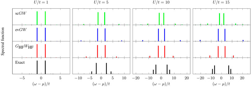
FIGURE 1. Spectral function of G (Eq. 3) as a function of (ω−μ)/t (where μ = U/2 is the chemical potential) at various values of the ratio U/t (U/t = 1, 5, 10, and 15) for different levels of theory: exact (black), G_HFW_HF (red), evGW (blue), and scGW (green). All approximate schemes are obtained using G_HF as starting point.

FIGURE 2

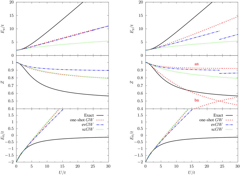
FIGURE 2. Fundamental gap (E_g), quasiparticle weight factors ($Z_{\text{bn}/\text{an}}^{\text{QP}}$), and ground state energy (E₀) as functions of U/t obtained from one-shot GW (dashed red line), evGW (dashed-dotted blue line), scGW (dotted green line) using G_HF (left) or G₀ (right) as starting point. The black curves are the exact results.

The main effects of full self-consistency are the reduction of E_g (see upper left panel of Figure 2), and the creation of extra satellites with decreasing intensity (see upper panel of Figure 1). For small U/t, the fundamental gap is similar to the one predicted by other methods while for increasing U/t the agreement worsen and E_g is grossly underestimated. The quasiparticle intensity is very similar to the one predicted by G_HFW_HF. Concerning the position of the satellites, we observe that the one-shot G_HFW_HF scheme gives the most promising results. Numerical values of quasiparticle and first satellite energies as well as their respective intensities in the spectral functions presented in Figure 1 are gathered in Table 1.

TABLE 1

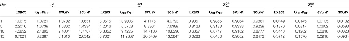
TABLE 1. Numerical values of quasiparticle energy ${ϵ}_{\text{an}}^{\text{QP}}$ and satellite energy ${ϵ}_{\text{an}}^{\text{sat}}$ (anti-bonding components) and respective intensities ($Z_{\text{an}}^{\text{QP}}$ and $Z_{\text{an}}^{\text{sat}}$) for the spectral functions presented in Figure 1. Energies are relative to the chemical potential μ = U/2. All spectral functions presented in Figure 1 are symmetric with respect to μ, which means that ${ϵ}_{\text{bn}}^{\text{QP/sat}}=-{ϵ}_{\text{an}}^{\text{QP/sat}}$ and $Z_{\text{bn}}^{\text{QP/sat}}=Z_{\text{an}}^{\text{QP/sat}}$.

We notice that a similar analysis for H₂ in a minimal basis has been presented in Ref. (Hellgren et al., 2015) with analogous conclusions.

For the sake of completeness, we also report in the bottom left panel of Figure 2 the total energy calculated using the Galitskii-Migdal formula (Eq. 4). Since the Galitskii-Migdal total energy is not stationary with respect to changes in G, one gets meaningful energies only at self-consistency. However, for the Hubbard dimer, we do not observe a significant impact of self-consistency, as one can see from Figure 1 by comparing the total energy at the G_HFW_HF, evGW, and scGW levels. For each of these schemes which correspond to a different level of self-consistency, the Galitskii-Migdal formula provides accurate total energies only for relatively small U/t (≲ 3).

If we consider G_HF as starting point and we define the chemical potential as $\mu =({ϵ}_{\text{an}}^{\text{QP}}+{ϵ}_{\text{bn}}^{\text{QP}})/2$, then the alignment of the chemical potential has no effect on the spectrum, this means that G_HFW_HF and pscGW are equivalent.

3.1.1 G₀: A Bad Starting Point

In the following we will illustrate how the starting point can influence the resulting quasiparticle energies. The Green’s function obtained from the one-shot G₀W₀ does not satisfy particle-hole symmetry, the fundamental gap is underestimated (top right panel of Figure 2) yet more accurate than G_HFW_HF (top left panel of Figure 2), the quasiparticle intensity relative to the bonding component is close to the exact result up to U/t ≈ 16 (center right panel of Figure 2), while overestimated for the antibonding components. Moreover, we note that the intensities of the two poles of the bonding component crosses at U/t = 24. This means that if we sort the quasiparticle and the satellite according to their intensity at a given U/t, the nature of the two poles is interchanged when one increases U/t, which results in a discontinuity in the QP energy. Meanwhile, the total number of particle is not conserved (N < 2). For G₀W₀ we found a small deviation from N = 2 for small U/t (e.g. N = 1.98828 at U = 1), which becomes larger by increasing the interaction (e.g. N = 1.55485 for U/t = 10). Instead, starting from G_HF the particle number is always conserved. We checked that for the self-consistent calculations the total particle number is conserved, as it should.

Considering G₀ as starting point in evGW, we encounter the problem described in Ref. (Véril et al., 2018), namely the discontinuity of various key properties (such as the fundamental gap in the top right panel of Figure 2) with respect to the interaction strength U/t. This issue is solved, for the Hubbard dimer, by considering a better starting point or using the fully self-consistent scheme scGW. Note, however, that improving the starting point does not always cure the discontinuity problem as this issue stems from the quasiparticle approximation itself. Full self-consistency, instead, avoids systematically discontinuities since no distinction is made between quasiparticle and satellites. Unfortunately, full self-consistency is much more involved from a computational point of view and, moreover, it does not give an overall improvement of the various properties of interest, at least for the Hubbard dimer, for which G_HFW_HF is to be preferred. For more realistic (molecular) systems, it was shown in Ref. (Berger et al., 2020). that the computationally cheaper self-consistent COHSEX scheme solves the problem of multiple quasiparticle solutions.

3.2 Bethe-Salpeter Equation

For the Hubbard dimer the matrices A^λ and B^λ in Eq. (8) are just single matrix elements and they simply read, for both spin manifolds,

$\begin{array}{llll}\hfill A^{\lambda ,\uparrow \downarrow }& =\mathrm{\Delta }{ϵ}^{GW}+\lambda \frac{U}{2},\hfill & \hfill B^{\lambda ,\uparrow \downarrow }& =\lambda \frac{U}{2}\left(\frac{4tU}{h^2}+1\right),\hfill \end{array}(\mathrm{26a})$

$\begin{array}{llll}\hfill A^{\lambda ,\uparrow \uparrow }& =\mathrm{\Delta }{ϵ}^{GW}-\lambda \frac{U}{2},\hfill & \hfill B^{\lambda ,\uparrow \uparrow }& =\lambda \frac{U}{2}\left(\frac{4tU}{h^2}-1\right),\hfill \end{array}(\mathrm{26b})$

while ${\tilde{A}}^{\lambda ,\uparrow \downarrow }=\lambda U$. We employ the screened Coulomb potential given in Eq. 22 at ω = 0 for the kernel, and the GW quasiparticle energies from Eqs 24a and 24b to build the GW approximation of the fundamental gap $\mathrm{\Delta }{ϵ}^{GW}={ϵ}_{\text{an}}^{\text{QP}}-{ϵ}_{\text{bn}}^{\text{QP}}$. For comparison purposes, we also use the exact quasiparticle energies [see Eq. (C3) of Ref. (Romaniello et al., 2012).], which consists in replacing Δε^GW by the exact fundamental gap $E_{\text{g}}=\sqrt{16t^2+U^2}-2t$. In such a case, one is able to specifically test how accurate the BSE formalism is at catching the excitonic effect via the introduction of the screened Coulomb potential.

We notice that, within the so-called Tamm-Dancoff approximation (TDA) where one neglects the coupling matrix B^λ between the resonant and anti-resonant parts of the BSE Hamiltonian (Eq. 8), BSE yields RPA with exchange (RPAx) excitation energies for the Hubbard dimer. This is the case also for approximations to the BSE kernel which are beyond GW, such as the T-matrix approximation. (Romaniello et al., 2012; Zhang et al., 2017; Li et al., 2021), and it is again related to the local nature of the electron-electron interaction. Hence, to test the effect of approximations on correlation for this model system we must go beyond the TDA.

3.2.1 Neutral Excitations

In Figure 3, we report the real part of the singlet and triplet excitation energies obtained from the solution of Eq. 8 for λ = 1. For comparison, we report also the exact excitation energies obtained as differences of the excited- and ground-state total energies of the Hubbard dimer obtained by diagonalizing the Hamiltonian (18) in the Slater determinant basis $\{\left|1\uparrow ,1\downarrow \right.⟩,\left|1\uparrow ,2\downarrow \right.⟩,\left|1\downarrow ,2\uparrow \right.⟩,\left|2\uparrow ,2\downarrow \right.⟩\}$ built from the sites [Ref. (Romaniello et al., 2009a) for the exact total energies]. For the singlet manifold, this yields, for the single excitation ${\mathrm{\Omega }}_1^{\uparrow \downarrow }$ and double excitation ${\mathrm{\Omega }}_2^{\uparrow \downarrow }$, the following expressions:

${\mathrm{\Omega }}_1^{\uparrow \downarrow }=\frac{1}{2}\left(U+\sqrt{16t^2+U^2}\right),{\mathrm{\Omega }}_2^{\uparrow \downarrow }=\sqrt{16t^2+U^2},(27)$

while the unique triplet transition energy is

${\mathrm{\Omega }}_1^{\uparrow \uparrow }=\frac{1}{2}\left(-U+\sqrt{16t^2+U^2}\right).(28)$

FIGURE 3

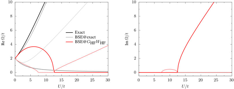
FIGURE 3. Real and imaginary parts of the singlet (solid) and triplet (dotted) neutral excitations, ${\mathrm{\Omega }}_1^{\uparrow \downarrow }$ and ${\mathrm{\Omega }}_1^{\uparrow \uparrow }$, as functions of U/t: exact (black), BSE with exact quasiparticle energies and W_HF (gray), BSE@G_HFW_HF (red).

Of course, one cannot access the double excitation within the static approximation of BSE, (Strinati, 1988; Romaniello et al., 2009b; Loos and Blase, 2020), so only the lowest singlet and triplet excitations, ${\mathrm{\Omega }}_1^{\uparrow \downarrow }$and ${\mathrm{\Omega }}_1^{\uparrow \uparrow }$, are studied below.

Using one-shot G_HFW_HF quasiparticle energies (BSE@G_HFW_HF) produces complex excitation energies (see right panel of Figure 3). We find the same scenario also with other flavors of GW (not reported in the figure), such as scGW. The occurrence of complex poles and singlet/triplet instabilities at the BSE level are well documented (Holzer et al., 2018; Blase et al., 2020; Loos et al., 2020) and is not specific to the Hubbard dimer. For example, one finds complex poles also for H₂ along its dissociation path, (Li and Olevano, 2021), but also for larger diatomic molecules. (Loos et al., 2020). For U/t > 12.4794, the singlet energy becomes pure imaginary, the same is observed for the triplet energy for 7.3524 < U/t < 12.4794. These two points corresponds to discontinuities in the first derivative of the excitation energies with respect to U/t (Figure 3). The BSE excitation energies are good approximations to their exact analogs only for U/t ≲ 2 for the singlet and U/t ≲ 6 for the triplet. Using exact quasiparticle energies instead produces real excitation energies, with the singlet energy in very good agreement with the exact result; the triplet energy, instead, largely overestimates the exact value. This seems to suggest that complex poles are caused by the approximate nature of the GW quasiparticle energies, although, of course, the quality of the kernel also plays a role. Indeed, setting W = 0 but using GW QP energies, BSE yields real-valued excitation energies. It would be interesting to further investigate this issue by using the exact kernel together with GW QP energies. This is left for future work.

3.2.2 Correlation Energy

For the Hubbard dimer, we have E^HF = − 2t + U/2, and the correlation energy given in Eq. 15 can be calculated analytically. After a lengthy but simple derivation, one gets

$\begin{array}{cc}\hfill E_{\text{c}}^{\text{AC@BSE}}& =-\frac{U}{2}+\frac{t^2-2U^2}{2U(2t+3U)}\left\{\mathrm{\Delta }{ϵ}^{GW}-\frac{1}{2(t+U)}\sqrt{[-U^2+2(t+U)\mathrm{\Delta }{ϵ}^{GW}]\left[U(2t+3U)+2(t+U)\mathrm{\Delta }{ϵ}^{GW}\right]}\right\}\hfill \\ \hfill & -\frac{t+2U}{2\sqrt{U(2t+3U)}}\left(\frac{3t+4U}{2t+3U}+\frac{t}{U}\right)\mathrm{\Delta }{ϵ}^{GW}\mathrm{a}\mathrm{t}\mathrm{a}\mathrm{n}\left\{-\frac{U\sqrt{U(2t+3U)}}{2\mathrm{\Delta }{ϵ}^{GW}(t+U)+\sqrt{[-U^2+2(t+U)\mathrm{\Delta }{ϵ}^{GW}][U(2t+3U)+2(t+U)\mathrm{\Delta }{ϵ}^{GW}]}}\right\}.\hfill \end{array}$

Results are reported in Figure 4 and are compared with the exact correlation energy (Romaniello et al., 2009a)

$E_{\text{c}}=-\frac{\sqrt{16t^2+U^2}}{2}+2t.(29)$

FIGURE 4

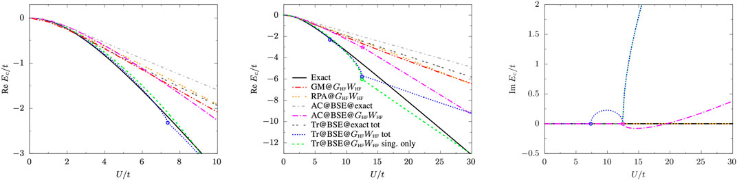
FIGURE 4. Real and imaginary parts of the BSE@G_HFW_HF correlation energy as a function of U/t at various levels of theory: total (dotted blue line) and singlet-only (dashed green line) Tr@BSE, AC@BSE (dot-dashed magenta line), RPA (triple-dotted orange line), GM (double-dot-dashed red line), and exact (solid black line). For comparison also the BSE@exact (Tr@BSE, double-dotted dark grey line; AC@BSE, dot-dashed light grey line) correlation energies are shown. Discontinuities in the first derivative of the energy (corresponding to the appearance of complex poles) are indicated by open circles.

The AC@BSE correlation energy does not possess the correct asymptotic behavior for small U, as Taylor expanding Eq. 29 for small U, we obtain

$E_{\text{c}}^{AC@BSE}=-\frac{U^2}{32t}-\frac{5U^3}{96t^2}+\frac{323U^4}{6144t^3}+\mathcal{O}(U^4),(30)$

while the exact correlation energy behaves as

$E_{\text{c}}=-\frac{U^2}{16t}+\frac{U^4}{1024t^3}+\mathcal{O}(U^6).(31)$

Moreover, we found that the radius of convergence of the small-U/t expansion of $E_{\text{c}}^{AC@BSE}$ is very small due to a square-root branch point for U/t ≈ − 2/3.

In the case of the trace formula Eq. 14, the singlet and triplet contributions behave as

$\begin{array}{ll}\hfill E_{\text{c},\uparrow \downarrow }^{\text{Tr@BSE}}& =-\frac{U^2}{32t}-\frac{7U^3}{128t^2}+\frac{99U^4}{2048t^3}+\mathcal{O}(U^5),\hfill \end{array}(\mathrm{32a})$

$\begin{array}{ll}\hfill E_{\text{c},\uparrow \uparrow }^{\text{Tr@BSE}}& =-\frac{U^2}{32t}+\frac{7U^3}{128t^2}-\frac{157U^4}{2048t^3}+\mathcal{O}(U^5),\hfill \end{array}(\mathrm{32b})$

which guarantees the correct asymptotic behavior for the total Tr@BSE correlation energy

$E_{\text{c}}^{\text{Tr@BSE}}=-\frac{U^2}{16t}-\frac{29U^4}{1024t^3}+\mathcal{O}(U^5),(33)$

and cancels the cubic term (as it should).

The trace formula is strongly affected by the appearance of the imaginary excitation energies: as shown in Figure 4 where we plot the real and complex components of the BSE@G_HFW_HF correlation energy as functions of U/t at various levels of theory, irregularities (i.e., discontinuities in the first derivative of the energy) appear at the values of U/t for which the triplet and singlet energies become purely imaginary. The ACFDT expression, instead, is more stable over the range of U/t considered here with only a small cusp on the energy surface at the singlet instability point after which the real part of E_c^AC@BSE behaves linearly with respect to U/t. Overall, however, the correlation energy obtained by the trace formula is almost on top of its exact counterpart over a wide range of U/t, with a rather small contribution from the triplet component, i.e., $\left|E_{\text{c},\uparrow \uparrow }^{\text{Tr@BSE}}\right|\ll \left|E_{\text{c},\uparrow \downarrow }^{\text{Tr@BSE}}\right|$. For comparison purposes, the RPA correlation energy, which is obtained from the trace or ACDFT formula using BSE@G_HFW_HF with W = 0 in the BSE kernel, is also reported in Figure 4. Both formulas yield the same correlation energies as expected, and they show no irregularities thanks to the fact that BSE excitation energies are real-valued at the RPA level. Also correlation energies obtained using BSE@exact (also shown in Figure 4) do not show irregularities for the same reason. Moreover, they show a visible upshift with respect to the corresponding AC@BSE@G_HFW_HF and Tr@BSE@G_HFW_HF results, which worsens the agreement with the exact correlation energy. Finally, we observe that both expressions for the correlation energy (at BSE@GW level) produce better results than the Galitskii-Migdal Eq. 4, as one can see from Figure 4, in particular at large U/t.

4 Conclusion

In this work we have used the symmetric Hubbard dimer to better understand some features of the GW approximation and of BSE@GW. In particular, we have found that the unphysical discontinuities that may occur in quasiparticle energies computed using one-shot or partially self-consistent GW schemes disappear using full self-consistency. However, full self-consistency does not give an overall improvement in term of accuracy and, at least for the Hubbard dimer, G_HFW_HF is to be preferred.

We have also analyzed the performance of the BSE@GW approach for neutral excitations and correlation energies. We have found that, at any level of self-consistency, the excitation energies become complex for some critical values of U/t. This seems related to the approximate nature of the GW quasiparticle energies, since using exact quasiparticle energies (hence the exact fundamental gap) solves this issue. The BSE excitation energies are good approximations to the exact analogs only for a small range of U/t (or U/t ≲ 2 for the lowest singlet-singlet transition and U/t ≲ 6 for the singlet-triplet transition), while the strong-correlation regime remains a challenge.

The correlation energy obtained from these excitation energies using the trace (or plasmon) formula has been found to be in very good agreement with the exact results over the whole range of U/t for which these energies are real. The occurrence of complex singlet and triplet excitation energies shows up as irregularities in the correlation energy. The ACFDT formula, instead, is less sensitive to this. However, we have found that the AC@BSE correlation energy is less accurate than the one obtained using the trace formula. Both, however, perform better than the standard Galitskii-Migdal formula. Finally, we have studied the small-U expansion of the correlation energy obtained with the trace and ACFDT formulas and we found that the former, contrary to the latter, has the correct behavior when one includes both the singlet and triplet energy contributions. Our findings point out to a possible fundamental problem of the AC@BSE formalism.

Although our study is restricted to the half-filled Hubbard dimer, some of our findings are transferable to realistic (molecular) systems. In particular: 1) a fully self-consistent solution of the GW equation cures the problem of multiple QP solutions, avoiding in the process the appearance of discontinuities in key physical quantities such as total or excitation energies, ionization potentials, and electron affinities; 2) a “bad” starting point (G₀ in the case of the Hubbard dimer) may result in the appearence of multiple QP solutions; 3) potential energy surfaces computed with the trace formula and within the ACFDT formalism may exhibit irregularities due to the appearence of complex BSE excitation energies; 4) for the Hubbard dimer at half-filling, the trace formula has the correct asymptotic behavior (thanks to the inclusion of singlet and triplet excitation energies) for weak interaction, contrary to its ACFDT counterpart. It would be interesting to check if it is also the case in realistic systems.

Data Availability Statement

The original contributions presented in the study are included in the article/Supplementary Material, further inquiries can be directed to the corresponding author.

Author Contributions

All authors listed have made a substantial, direct, and intellectual contribution to the work and approved it for publication.

Funding

This study has been partially supported through the EUR grant NanoX no ANR-17-EURE-0009 in the framework of the “Programme des Investissements d’Avenir” and by the CNRS through the 80|Prime program. PR and SDS also thank the ANR (project ANR-18-CE30-0025) for financial support. PFL also thanks the European Research Council (ERC) under the European Union’s Horizon 2020 research and innovation programme (grant agreement no. ∼863481) for financial support.

Conflict of Interest

The authors declare that the research was conducted in the absence of any commercial or financial relationships that could be construed as a potential conflict of interest.

Publisher’s Note

All claims expressed in this article are solely those of the authors and do not necessarily represent those of their affiliated organizations or those of the publisher, the editors, and the reviewers. Any product that may be evaluated in this article or claim that may be made by its manufacturer is not guaranteed or endorsed by the publisher.

Supplementary Material

The Supplementary Material for this article can be found online at: https://www.frontiersin.org/articles/10.3389/fchem.2021.751054/full#supplementary-material

References

Albrecht, S., Reining, L., Del Sole, R., and Onida, G. (1998). Ab InitioCalculation of Excitonic Effects in the Optical Spectra of Semiconductors. Phys. Rev. Lett. 80, 4510–4513. doi:10.1103/PhysRevLett.80.4510

CrossRef Full Text | Google Scholar

Ángyán, J. G., Liu, R.-F., Toulouse, J., and Jansen, G. (2011). Correlation Energy Expressions from the Adiabatic-Connection Fluctuation-Dissipation Theorem Approach. J. Chem. Theor. Comput. 7, 3116–3130. doi:10.1021/ct200501r

CrossRef Full Text | Google Scholar

Aryasetiawan, F., and Gunnarsson, O. (1998). TheGWmethod. Rep. Prog. Phys. 61, 237–312. doi:10.1088/0034-4885/61/3/002

CrossRef Full Text | Google Scholar

Authier, J., and Loos, P.-F. (2020). Dynamical Kernels for Optical Excitations. J. Chem. Phys. 153, 184105. doi:10.1063/5.0028040

CrossRef Full Text | Google Scholar

Benedict, L. X., Shirley, E. L., and Bohn, R. B. (1998). Optical Absorption of Insulators and the Electron-Hole Interaction: AnAb InitioCalculation. Phys. Rev. Lett. 80, 4514–4517. doi:10.1103/PhysRevLett.80.4514

CrossRef Full Text | Google Scholar

Berger, J. A., Loos, P.-F., and Romaniello, P. (2020). Potential Energy Surfaces without Unphysical Discontinuities: The Coulomb Hole Plus Screened Exchange Approach. J. Chem. Theor. Comput. 17, 191–200. doi:10.1021/acs.jctc.0c00896

PubMed Abstract | CrossRef Full Text | Google Scholar

Blase, X., and Attaccalite, C. (2011). Charge-transfer Excitations in Molecular Donor-Acceptor Complexes within the many-body Bethe-Salpeter Approach. Appl. Phys. Lett. 99, 171909. doi:10.1063/1.3655352

CrossRef Full Text | Google Scholar

Blase, X., Boulanger, P., Bruneval, F., Fernandez-Serra, M., and Duchemin, I. (2016). GW and Bethe-Salpeter Study of Small Water Clusters. J. Chem. Phys. 144, 034109. doi:10.1063/1.4940139

CrossRef Full Text | Google Scholar

Blase, X., Duchemin, I., Jacquemin, D., and Loos, P.-F. (2020). The Bethe-Salpeter Equation Formalism: From Physics to Chemistry. J. Phys. Chem. Lett. 11, 7371–7382. doi:10.1021/acs.jpclett.0c01875

PubMed Abstract | CrossRef Full Text | Google Scholar

Blase, X., Duchemin, I., and Jacquemin, D. (2018). The Bethe-Salpeter Equation in Chemistry: Relations with TD-DFT, Applications and Challenges. Chem. Soc. Rev. 47, 1022–1043. doi:10.1039/C7CS00049A

PubMed Abstract | CrossRef Full Text | Google Scholar

Boulanger, P., Jacquemin, D., Duchemin, I., and Blase, X. (2014). Fast and Accurate Electronic Excitations in Cyanines with the many-body Bethe-Salpeter Approach. J. Chem. Theor. Comput. 10, 1212–1218. doi:10.1021/ct401101u

PubMed Abstract | CrossRef Full Text | Google Scholar

Bruneval, F., Hamed, S. M., and Neaton, J. B. (2015). A Systematic Benchmark of the ab initio Bethe-Salpeter Equation Approach for Low-Lying Optical Excitations of Small Organic Molecules. J. Chem. Phys. 142, 244101. doi:10.1063/1.4922489

CrossRef Full Text | Google Scholar

Bruneval, F. (2012). Ionization Energy of Atoms Obtained from GW Self-Energy or from Random Phase Approximation Total Energies. J. Chem. Phys. 136, 194107. doi:10.1063/1.4718428

CrossRef Full Text | Google Scholar

Bruneval, F., and Marques, M. A. L. (2013). Benchmarking the Starting Points of the GW Approximation for Molecules. J. Chem. Theor. Comput. 9, 324–329. doi:10.1021/ct300835h

PubMed Abstract | CrossRef Full Text | Google Scholar

Bruneval, F. (2016). Optimized Virtual Orbital Subspace for Faster GW Calculations in Localized Basis. J. Chem. Phys. 145, 234110. doi:10.1063/1.4972003

CrossRef Full Text | Google Scholar

Bruneval, F., Rangel, T., Hamed, S. M., Shao, M., Yang, C., and Neaton, J. B. (2016). Molgw 1: Many-body Perturbation Theory Software for Atoms, Molecules, and Clusters. Computer Phys. Commun. 208, 149–161. doi:10.1016/j.cpc.2016.06.019

CrossRef Full Text | Google Scholar

Carrascal, D. J., Ferrer, J., Maitra, N., and Burke, K. (2018). Linear Response Time-dependent Density Functional Theory of the Hubbard Dimer. Eur. Phys. J. B 91, 142. doi:10.1140/epjb/e2018-90114-9

CrossRef Full Text | Google Scholar

Carrascal, D. J., Ferrer, J., Smith, J. C., and Burke, K. (2015). The Hubbard Dimer: A Density Functional Case Study of a many-body Problem. J. Phys. Condens. Matter 27, 393001. doi:10.1088/0953-8984/27/39/393001

CrossRef Full Text | Google Scholar

Caruso, F., Rinke, P., Ren, X., Rubio, A., and Scheffler, M. (2013a). Self-consistentGW: All-Electron Implementation with Localized Basis Functions. Phys. Rev. B 88, 075105. doi:10.1103/PhysRevB.88.075105

CrossRef Full Text | Google Scholar

Caruso, F., Rinke, P., Ren, X., Scheffler, M., and Rubio, A. (2012). Unified Description of Ground and Excited States of Finite Systems: The Self-consistentGWapproach. Phys. Rev. B 86, 081102. doi:10.1103/PhysRevB.86.081102

CrossRef Full Text | Google Scholar

Caruso, F., Rohr, D. R., Hellgren, M., Ren, X., Rinke, P., Rubio, A., et al. (2013b). Bond Breaking and Bond Formation: How Electron Correlation Is Captured in Many-Body Perturbation Theory and Density-Functional Theory. Phys. Rev. Lett. 110, 146403. doi:10.1103/PhysRevLett.110.146403

PubMed Abstract | CrossRef Full Text | Google Scholar

Caruso, F. (2013). “Self-Consistent GW Approach for the Unified Description of Ground and Excited States of Finite Systems,”. PhD Thesis (Berlin, Germany: Freie Universität Berlin).

Google Scholar

Casida, M. E. (1995). Generalization of the Optimized-Effective-Potential Model to Include Electron Correlation: A Variational Derivation of the Sham-Schlüter Equation for the Exact Exchange-Correlation Potential. Phys. Rev. A. 51, 2005–2013. doi:10.1103/PhysRevA.51.2005

PubMed Abstract | CrossRef Full Text | Google Scholar

Casida, M. E., and Huix-Rotllant, M. (2015). Many-body Perturbation Theory (MBPT) and Time-dependent Density-Functional Theory (TD-DFT): MBPT Insights about what Is Missing in, and Corrections to, the TD-DFT Adiabatic Approximation. Top. Curr. Chem. 368, 1–60. doi:10.1007/128_2015_632

PubMed Abstract | CrossRef Full Text | Google Scholar

Casida, M. E. (2005). Propagator Corrections to Adiabatic Time-dependent Density-Functional Theory Linear Response Theory. J. Chem. Phys. 122, 054111. doi:10.1063/1.1836757

CrossRef Full Text | Google Scholar

Colonna, N., Hellgren, M., and de Gironcoli, S. (2014). Correlation Energy within Exact-Exchange Adiabatic Connection Fluctuation-Dissipation Theory: Systematic Development and Simple Approximations. Phys. Rev. B 90, 125150. doi:10.1103/physrevb.90.125150

CrossRef Full Text | Google Scholar

Di Sabatino, S., Berger, J. A., Reining, L., and Romaniello, P. (2016). Photoemission Spectra from Reduced Density Matrices: The Band gap in Strongly Correlated Systems. Phys. Rev. B 94, 155141. doi:10.1103/PhysRevB.94.155141

CrossRef Full Text | Google Scholar

Dreuw, A., and Head-Gordon, M. (2005). Single-Reference Ab Initio Methods for the Calculation of Excited States of Large Molecules. Chem. Rev. 105, 4009–4037. doi:10.1021/cr0505627

PubMed Abstract | CrossRef Full Text | Google Scholar

Duchemin, I., and Blase, X. (2021). Cubic-Scaling All-Electron GW Calculations with a Separable Density-Fitting Space-Time Approach. J. Chem. Theor. Comput. 17, 2383–2393. doi:10.1021/acs.jctc.1c00101

CrossRef Full Text | Google Scholar

Duchemin, I., and Blase, X. (2020). Robust Analytic-Continuation Approach to many-body GW Calculations. J. Chem. Theor. Comput. 16, 1742–1756. doi:10.1021/acs.jctc.9b01235

PubMed Abstract | CrossRef Full Text | Google Scholar

Duchemin, I., and Blase, X. (2019). Separable Resolution-Of-The-Identity with All-Electron Gaussian Bases: Application to Cubic-Scaling Rpa. J. Chem. Phys. 150, 174120. doi:10.1063/1.5090605

CrossRef Full Text | Google Scholar

Faber, C., Attaccalite, C., Olevano, V., Runge, E., and Blase, X. (2011). First-principlesGWcalculations for DNA and RNA Nucleobases. Phys. Rev. B 83, 115123. doi:10.1103/PhysRevB.83.115123

CrossRef Full Text | Google Scholar

Faber, C. (2014). “Electronic, Excitonic and Polaronic Properties of Organic Systems within the Many-Body GW and Bethe-Salpeter Formalisms: Towards Organic Photovoltaics,”. PhD Thesis (Grenoble, France: Université de Grenoble).

Google Scholar

Furche, F., and Van Voorhis, T. (2005). Fluctuation-dissipation Theorem Density-Functional Theory. J. Chem. Phys. 122, 164106. doi:10.1063/1.1884112

CrossRef Full Text | Google Scholar

Galitskii, V., and Migdal, A. (1958). Applications of Quantum Field Theory to the many Body Problem. Sov. Phys. JETP 7, 96.

Google Scholar

Golze, D., Dvorak, M., and Rinke, P. (2019). The Gw Compendium: A Practical Guide to Theoretical Photoemission Spectroscopy. Front. Chem. 7, 377. doi:10.3389/fchem.2019.00377

PubMed Abstract | CrossRef Full Text | Google Scholar

Gui, X., Holzer, C., and Klopper, W. (2018). Accuracy Assessment of GW Starting Points for Calculating Molecular Excitation Energies Using the Bethe-Salpeter Formalism. J. Chem. Theor. Comput. 14, 2127–2136. doi:10.1021/acs.jctc.8b00014

PubMed Abstract | CrossRef Full Text | Google Scholar

Gunnarsson, O., and Lundqvist, B. I. (1976). Exchange and Correlation in Atoms, Molecules, and Solids by the Spin-Density-Functional Formalism. Phys. Rev. B 13, 4274–4298. doi:10.1103/PhysRevB.13.4274

CrossRef Full Text | Google Scholar

Hedin, L. (1965). New Method for Calculating the One-Particle Green's Function with Application to the Electron-Gas Problem. Phys. Rev. 139, A796–A823. doi:10.1103/physrev.139.a796

CrossRef Full Text | Google Scholar

Hellgren, M., Caruso, F., Rohr, D. R., Ren, X., Rubio, A., Scheffler, M., et al. (2015). Static Correlation and Electron Localization in Molecular Dimers from the Self-Consistent RPA andGWapproximation. Phys. Rev. B 91, 165110. doi:10.1103/physrevb.91.165110

CrossRef Full Text | Google Scholar

Hellgren, M., and von Barth, U. (2010). Correlation Energy Functional and Potential from Time-dependent Exact-Exchange Theory. J. Chem. Phys. 132, 044101. doi:10.1063/1.3290947

CrossRef Full Text | Google Scholar

Heßelmann, A., and Görling, A. (2011). Correct Description of the Bond Dissociation Limit without Breaking Spin Symmetry by a Random-Phase-Approximation Correlation Functional. Phys. Rev. Lett. 106, 093001. doi:10.1103/PhysRevLett.106.093001

PubMed Abstract | CrossRef Full Text | Google Scholar

Hirose, D., Noguchi, Y., and Sugino, O. (2015). All-electronGW+Bethe-Salpeter Calculations on Small Molecules. Phys. Rev. B 91, 205111. doi:10.1103/physrevb.91.205111

CrossRef Full Text | Google Scholar

Hohenberg, P., and Kohn, W. (1964). Inhomogeneous Electron Gas. Phys. Rev. 136, B864–B871. doi:10.1103/PhysRev.136.B864

CrossRef Full Text | Google Scholar

Holm, B., and von Barth, U. (1998). Fully Self-consistentGWself-Energy of the Electron Gas. Phys. Rev. B 57, 2108–2117. doi:10.1103/PhysRevB.57.2108

CrossRef Full Text | Google Scholar

Holzer, C., Gui, X., Harding, M. E., Kresse, G., Helgaker, T., and Klopper, W. (2018). Bethe-Salpeter Correlation Energies of Atoms and Molecules. J. Chem. Phys. 149, 144106. doi:10.1063/1.5047030

CrossRef Full Text | Google Scholar

Holzer, C., and Klopper, W. (2018). Communication: A Hybrid Bethe-salpeter/time-dependent Density-Functional-Theory Approach for Excitation Energies. J. Chem. Phys. 149, 101101. doi:10.1063/1.5051028

CrossRef Full Text | Google Scholar

Huix-Rotllant, M., Ipatov, A., Rubio, A., and Casida, M. E. (2011). Assessment of Dressed Time-dependent Density-Functional Theory for the Low-Lying Valence States of 28 Organic Chromophores. Chem. Phys. 391, 120–129. doi:10.1016/j.chemphys.2011.03.019

CrossRef Full Text | Google Scholar

Hung, L., Bruneval, F., Baishya, K., and Öğüt, S. (2017). Benchmarking the GW Approximation and Bethe-Salpeter Equation for Groups IB and IIB Atoms and Monoxides. J. Chem. Theor. Comput. 13, 2135–2146. doi:10.1021/acs.jctc.7b00123

PubMed Abstract | CrossRef Full Text | Google Scholar

Hung, L., da Jornada, F. H., Souto-Casares, J., Chelikowsky, J. R., Louie, S. G., and Öğüt, S. (2016). Excitation Spectra of Aromatic Molecules within a Real-spaceGW-BSE Formalism: Role of Self-Consistency and Vertex Corrections. Phys. Rev. B 94, 085125. doi:10.1103/PhysRevB.94.085125

CrossRef Full Text | Google Scholar

Hybertsen, M. S., and Louie, S. G. (1986). Electron Correlation in Semiconductors and Insulators: Band Gaps and Quasiparticle Energies. Phys. Rev. B 34, 5390–5413. doi:10.1103/PhysRevB.34.5390

PubMed Abstract | CrossRef Full Text | Google Scholar

Jacquemin, D., Duchemin, I., and Blase, X. (2015a). 0-0 Energies Using Hybrid Schemes: Benchmarks of TD-DFT, CIS(D), ADC(2), CC2, and BSE/GW Formalisms for 80 Real-Life Compounds. J. Chem. Theor. Comput. 11, 5340–5359. doi:10.1021/acs.jctc.5b00619

PubMed Abstract | CrossRef Full Text | Google Scholar

Jacquemin, D., Duchemin, I., and Blase, X. (2015b). Benchmarking the Bethe-Salpeter Formalism on a Standard Organic Molecular Set. J. Chem. Theor. Comput. 11, 3290–3304. doi:10.1021/acs.jctc.5b00304

PubMed Abstract | CrossRef Full Text | Google Scholar

Jacquemin, D., Duchemin, I., and Blase, X. (2017a). Is the Bethe-Salpeter Formalism Accurate for Excitation Energies? Comparisons with TD-DFT, CASPT2, and EOM-CCSD. J. Phys. Chem. Lett. 8, 1524–1529. doi:10.1021/acs.jpclett.7b00381

PubMed Abstract | CrossRef Full Text | Google Scholar

Jacquemin, D., Duchemin, I., Blondel, A., and Blase, X. (2017b). Benchmark of Bethe-Salpeter for Triplet Excited-States. J. Chem. Theor. Comput. 13, 767–783. doi:10.1021/acs.jctc.6b01169

PubMed Abstract | CrossRef Full Text | Google Scholar

Kaplan, F., Harding, M. E., Seiler, C., Weigend, F., Evers, F., and van Setten, M. J. (2016). Quasi-Particle Self-Consistent GW for Molecules. J. Chem. Theor. Comput. 12, 2528–2541. doi:10.1021/acs.jctc.5b01238

PubMed Abstract | CrossRef Full Text | Google Scholar

Kaplan, F., Weigend, F., Evers, F., and van Setten, M. J. (2015). Off-Diagonal Self-Energy Terms and Partially Self-Consistency in GW Calculations for Single Molecules: Efficient Implementation and Quantitative Effects on Ionization Potentials. J. Chem. Theor. Comput. 11, 5152–5160. doi:10.1021/acs.jctc.5b00394

PubMed Abstract | CrossRef Full Text | Google Scholar

Karlsson, D., and van Leeuwen, R. (2016). Partial Self-Consistency and Analyticity in many-body Perturbation Theory: Particle Number Conservation and a Generalized Sum Rule. Phys. Rev. B 94, 125124. doi:10.1103/PhysRevB.94.125124

CrossRef Full Text | Google Scholar

Kohn, W., and Sham, L. J. (1965). Self-consistent Equations Including Exchange and Correlation Effects. Phys. Rev. 140, A1133–A1138. doi:10.1103/PhysRev.140.A1133

CrossRef Full Text | Google Scholar

Koval, P., Foerster, D., and Sánchez-Portal, D. (2014). Fully Self-consistentGWand Quasiparticle Self-consistentGWfor Molecules. Phys. Rev. B 89, 155417. doi:10.1103/PhysRevB.89.155417

CrossRef Full Text | Google Scholar

Krause, K., and Klopper, W. (2017). Implementation of the Bethe−Salpeter Equation in the TURBOMOLE Program. J. Comput. Chem. 38, 383–388. doi:10.1002/jcc.24688

PubMed Abstract | CrossRef Full Text | Google Scholar

Langreth, D. C., and Perdew, J. P. (1979). The Gradient Approximation to the Exchange-Correlation Energy Functional: A Generalization that Works. Solid State. Commun. 31, 567–571. doi:10.1016/0038-1098(79)90254-0

CrossRef Full Text | Google Scholar

Lettmann, T., and Rohlfing, M. (2019). Electronic Excitations of Polythiophene within many-body Perturbation Theory with and without the Tamm-Dancoff Approximation. J. Chem. Theor. Comput. 15, 4547–4554. doi:10.1021/acs.jctc.9b00223

PubMed Abstract | CrossRef Full Text | Google Scholar

Li, J., Chen, Z., and Yang, W. (2021). Renormalized Singles Green's Function in the T-Matrix Approximation for Accurate Quasiparticle Energy Calculation. J. Phys. Chem. Lett. 12, 6203–6210. doi:10.1021/acs.jpclett.1c01723

CrossRef Full Text | Google Scholar

Li, J., Drummond, N. D., Schuck, P., and Olevano, V. (2019). Comparing many-body Approaches against the Helium Atom Exact Solution. Scipost Phys. 6, 040. doi:10.21468/SciPostPhys.6.4.040

CrossRef Full Text | Google Scholar

Li, J., Duchemin, I., Blase, X., and Olevano, V. (2020). Ground-state Correlation Energy of Beryllium Dimer by the Bethe-Salpeter Equation. Scipost Phys. 8, 20. doi:10.21468/SciPostPhys.8.2.020

CrossRef Full Text | Google Scholar

Li, J., Holzmann, M., Duchemin, I., Blase, X., and Olevano, V. (2017). Helium Atom Excitations by the GW and Bethe-Salpeter Many-Body Formalism. Phys. Rev. Lett. 118, 163001. doi:10.1103/PhysRevLett.118.163001

PubMed Abstract | CrossRef Full Text | Google Scholar

Li, J., and Olevano, V. (2021). Hydrogen-molecule Spectrum by the many-body Gw Approximation and the Bethe-Salpeter Equation. Phys. Rev. A. 103, 012809. doi:10.1103/PhysRevA.103.012809

CrossRef Full Text | Google Scholar

Liu, C., Kloppenburg, J., Yao, Y., Ren, X., Appel, H., Kanai, Y., et al. (2020). All-electron ab initio Bethe-Salpeter Equation Approach to Neutral Excitations in Molecules with Numeric Atom-Centered Orbitals. J. Chem. Phys. 152, 044105. doi:10.1063/1.5123290

PubMed Abstract | CrossRef Full Text | Google Scholar

Loos, P.-F., and Blase, X. (2020). Dynamical Correction to the Bethe-Salpeter Equation beyond the Plasmon-Pole Approximation. J. Chem. Phys. 153, 114120. doi:10.1063/5.0023168

CrossRef Full Text | Google Scholar

Loos, P.-F., Romaniello, P., and Berger, J. A. (2018). Green Functions and Self-Consistency: Insights from the Spherium Model. J. Chem. Theor. Comput. 14, 3071–3082. doi:10.1021/acs.jctc.8b00260

PubMed Abstract | CrossRef Full Text | Google Scholar

Loos, P.-F., Scemama, A., Duchemin, I., Jacquemin, D., and Blase, X. (2020). Pros and Cons of the Bethe-Salpeter Formalism for Ground-State Energies. J. Phys. Chem. Lett. 11, 3536–3545. doi:10.1021/acs.jpclett.0c00460

PubMed Abstract | CrossRef Full Text | Google Scholar

Ma, Y., Rohlfing, M., and Molteni, C. (2009a). Excited States of Biological Chromophores Studied Using many-body Perturbation Theory: Effects of Resonant-Antiresonant Coupling and Dynamical Screening. Phys. Rev. B 80, 241405. doi:10.1103/PhysRevB.80.241405

CrossRef Full Text | Google Scholar

Ma, Y., Rohlfing, M., and Molteni, C. (2009b). Modeling the Excited States of Biological Chromophores within Many-Body Green's Function Theory. J. Chem. Theor. Comput. 6, 257–265. doi:10.1021/ct900528h

PubMed Abstract | CrossRef Full Text | Google Scholar

Maggio, E., and Kresse, G. (2016). Correlation Energy for the Homogeneous Electron Gas: Exact Bethe-Salpeter Solution and an Approximate Evaluation. Phys. Rev. B 93, 235113. doi:10.1103/PhysRevB.93.235113

CrossRef Full Text | Google Scholar

Maggio, E., Liu, P., van Setten, M. J., and Kresse, G. (2017). GW100: A Plane Wave Perspective for Small Molecules. J. Chem. Theor. Comput. 13, 635–648. doi:10.1021/acs.jctc.6b01150

PubMed Abstract | CrossRef Full Text | Google Scholar

Martin, R. M., Reining, L., and Ceperley, D. (2016). Interacting Electrons: Theory and Computational Approaches. New York, NY: Cambridge University Press.

Google Scholar

Monino, E., and Loos, P.-F. (2021). Spin-Conserved and Spin-Flip Optical Excitations from the Bethe-Salpeter Equation Formalism. J. Chem. Theor. Comput. 17, 2852–2867. doi:10.1021/acs.jctc.1c00074

CrossRef Full Text | Google Scholar

Myöhänen, P., Stan, A., Stefanucci, G., and van Leeuwen, R. (2008). A many-body Approach to Quantum Transport Dynamics: Initial Correlations and Memory Effects. Europhys. Lett. 84, 67001. doi:10.1209/0295-5075/84/67001

CrossRef Full Text | Google Scholar

Oddershede, J., and Jo/rgensen, P. (1977). An Order Analysis of the Particle-Hole Propagator. J. Chem. Phys. 66, 1541–1556. doi:10.1063/1.434118

CrossRef Full Text | Google Scholar

Olevano, V., Toulouse, J., and Schuck, P. (2019). A Formally Exact One-Frequency-Only Bethe-salpeter-like Equation. Similarities and Differences between Gw+bse and Self-Consistent Rpa. J. Chem. Phys. 150, 084112. doi:10.1063/1.5080330

CrossRef Full Text | Google Scholar

Olsen, T., and Thygesen, K. S. (2014). Static Correlation beyond the Random Phase Approximation: Dissociating H2 with the Bethe-Salpeter Equation and Time-dependent Gw. J. Chem. Phys. 140, 164116. doi:10.1063/1.4871875

PubMed Abstract | CrossRef Full Text | Google Scholar

Onida, G., Reining, L., and Rubio, A. (2002). Electronic Excitations: Density-Functional versus many-body green’s Function Approaches. Rev. Mod. Phys. 74, 601–659. doi:10.1103/RevModPhys.74.601

CrossRef Full Text | Google Scholar

Ou, Q., and Subotnik, J. E. (2016). Comparison between GW and Wave-Function-Based Approaches: Calculating the Ionization Potential and Electron Affinity for 1D Hubbard Chains. J. Phys. Chem. A. 120, 4514–4525. doi:10.1021/acs.jpca.6b03294

PubMed Abstract | CrossRef Full Text | Google Scholar

Ou, Q., and Subotnik, J. E. (2018). Comparison between the Bethe–Salpeter Equation and Configuration Interaction Approaches for Solving a Quantum Chemistry Problem: Calculating the Excitation Energy for Finite 1D Hubbard Chains. J. Chem. Theor. Comput. 14, 527–542. doi:10.1021/acs.jctc.7b00246

PubMed Abstract | CrossRef Full Text | Google Scholar

Petersilka, M., Gossmann, U. J., and Gross, E. K. U. (1996). Excitation Energies from Time-dependent Density-Functional Theory. Phys. Rev. Lett. 76, 1212. doi:10.1103/PhysRevLett.76.1212

PubMed Abstract | CrossRef Full Text | Google Scholar

Pollehn, T. J., Schindlmayr, A., and Godby, R. W. (1998). Assessment of theGWapproximation Using hubbard Chains. J. Phys. Condensed Matter 10, 1273–1283. doi:10.1088/0953-8984/10/6/011

CrossRef Full Text | Google Scholar

Puig von Friesen, M., Verdozzi, C., and Almbladh, C.-O. (2010). Kadanoff-baym Dynamics of hubbard Clusters: Performance of many-body Schemes, Correlation-Induced Damping and Multiple Steady and Quasi-Steady States. Phys. Rev. B 82, 155108. doi:10.1103/PhysRevB.82.155108

CrossRef Full Text | Google Scholar

Puschnig, P., and Ambrosch-Draxl, C. (2002). Suppression of Electron-Hole Correlations in 3d Polymer Materials. Phys. Rev. Lett. 89, 056405. doi:10.1103/PhysRevLett.89.056405

PubMed Abstract | CrossRef Full Text | Google Scholar

Rangel, T., Hamed, S. M., Bruneval, F., and Neaton, J. B. (2017). An Assessment of Low-Lying Excitation Energies and Triplet Instabilities of Organic Molecules with an ab initio Bethe-Salpeter Equation Approach and the Tamm-Dancoff Approximation. J. Chem. Phys. 146, 194108. doi:10.1063/1.4983126

PubMed Abstract | CrossRef Full Text | Google Scholar

Rangel, T., Hamed, S. M., Bruneval, F., and Neaton, J. B. (2016). Evaluating the Gw Approximation with Ccsd(t) for Charged Excitations across the Oligoacenes. J. Chem. Theor. Comput. 12, 2834–2842. doi:10.1021/acs.jctc.6b00163

PubMed Abstract | CrossRef Full Text | Google Scholar

Rebolini, E., and Toulouse, J. (2016). Range-separated Time-dependent Density-Functional Theory with a Frequency-dependent Second-Order Bethe-Salpeter Correlation Kernel. J. Chem. Phys. 144, 094107. doi:10.1063/1.4943003

CrossRef Full Text | Google Scholar

Ring, P., and Schuck, P. (1980). The Nuclear Many-Body Problem. New York: Springer-Verlag.

Google Scholar

Rohlfing, M., and Louie, S. G. (2000). Electron-hole Excitations and Optical Spectra from First Principles. Phys. Rev. B 62, 4927–4944. doi:10.1103/PhysRevB.62.4927

CrossRef Full Text | Google Scholar

Rohlfing, M., and Louie, S. G. (1998). Electron-hole Excitations in Semiconductors and Insulators. Phys. Rev. Lett. 81, 2312–2315. doi:10.1103/PhysRevLett.81.2312

CrossRef Full Text | Google Scholar

Rohlfing, M., and Louie, S. G. (1999). Optical Excitations in Conjugated Polymers. Phys. Rev. Lett. 82, 1959–1962. doi:10.1103/PhysRevLett.82.1959

CrossRef Full Text | Google Scholar

Romaniello, P., Bechstedt, F., and Reining, L. (2012). Beyond the G W Approximation: Combining Correlation Channels. Phys. Rev. B 85, 155131. doi:10.1103/PhysRevB.85.155131

CrossRef Full Text | Google Scholar

Romaniello, P., Guyot, S., and Reining, L. (2009a). The Self-Energy beyond GW: Local and Nonlocal Vertex Corrections. J. Chem. Phys. 131, 154111. doi:10.1063/1.3249965

CrossRef Full Text | Google Scholar

Romaniello, P., Sangalli, D., Berger, J. A., Sottile, F., Molinari, L. G., Reining, L., et al. (2009b). Double Excitations in Finite Systems. J. Chem. Phys. 130, 044108. doi:10.1063/1.3065669

CrossRef Full Text | Google Scholar

Rowe, D. J. (1968). Methods for Calculating Ground-State Correlations of Vibrational Nuclei. Phys. Rev. 175, 1283. doi:10.1103/PhysRev.175.1283

CrossRef Full Text | Google Scholar

Runge, E., and Gross, E. K. U. (1984). Density-functional Theory for Time-dependent Systems. Phys. Rev. Lett. 52, 997–1000. doi:10.1103/PhysRevLett.52.997

CrossRef Full Text | Google Scholar

Sakkinen, N., Manninen, M., and van Leeuwen, R. (2012). The Kadanoff-Baym Approach to Double Excitations in Finite Systems. New J. Phys. 14, 013032. doi:10.1088/1367-2630/14/1/013032

CrossRef Full Text | Google Scholar

Salpeter, E. E., and Bethe, H. A. (1951). A Relativistic Equation for Bound-State Problems. Phys. Rev. 84, 1232. doi:10.1103/PhysRev.84.1232

CrossRef Full Text | Google Scholar

Sangalli, D., Romaniello, P., Onida, G., and Marini, A. (2011). Double Excitations in Correlated Systems: A many–body Approach. J. Chem. Phys. 134, 034115. doi:10.1063/1.3518705

CrossRef Full Text | Google Scholar

Schindlmayr, A., Pollehn, T. J., and Godby, R. W. (1998). Spectra and Total Energies from Self-Consistent many-body Perturbation Theory. Phys. Rev. B 58, 12684–12690. doi:10.1103/PhysRevB.58.12684

CrossRef Full Text | Google Scholar

Schindlmayr, A. (1997). Violation of Particle Number Conservation in the GW Approximation. Phys. Rev. B 56, 3528–3531. doi:10.1103/PhysRevB.56.3528

CrossRef Full Text | Google Scholar

Shishkin, M., and Kresse, G. (2007). Self-consistent G W Calculations for Semiconductors and Insulators. Phys. Rev. B 75, 235102. doi:10.1103/PhysRevB.75.235102

CrossRef Full Text | Google Scholar

Sottile, F., Olevano, V., and Reining, L. (2003). Parameter-free Calculation of Response Functions in Time-dependent Density-Functional Theory. Phys. Rev. Lett. 91, 056402. doi:10.1103/PhysRevLett.91.056402

PubMed Abstract | CrossRef Full Text | Google Scholar

Stan, A., Dahlen, N. E., and van Leeuwen, R. (2006). Fully Self-Consistent GW Calculations for Atoms and Molecules. Europhys. Lett. EPL 76, 298–304. doi:10.1209/epl/i2006-10266-6

CrossRef Full Text | Google Scholar

Stan, A., Dahlen, N. E., and van Leeuwen, R. (2009). Levels of Self-Consistency in the Gw Approximation. J. Chem. Phys. 130, 114105. doi:10.1063/1.3089567

CrossRef Full Text | Google Scholar

Strinati, G. (1988). Application of the Green’s Functions Method to the Study of the Optical Properties of Semiconductors. Riv. Nuovo Cimento 11, 1–86. doi:10.1007/BF02725962

CrossRef Full Text | Google Scholar

Szabo, A., and Ostlund, N. S. (1989). Modern Quantum Chemistry. New York: McGraw-Hill.

Google Scholar

Tiago, M. L., Northrup, J. E., and Louie, S. G. (2003). Ab Initio calculation of the Electronic and Optical Properties of Solid Pentacene. Phys. Rev. B 67, 115212. doi:10.1103/PhysRevB.67.115212

CrossRef Full Text | Google Scholar

Toulouse, J., Gerber, I. C., Jansen, G., Savin, A., and Angyan, J. G. (2009). Adiabatic-connection Fluctuation-Dissipation Density-Functional Theory Based on Range Separation. Phys. Rev. Lett. 102, 096404. doi:10.1103/PhysRevLett.102.096404

PubMed Abstract | CrossRef Full Text | Google Scholar

Toulouse, J., Zhu, W., Angyan, J. G., and Savin, A. (2010). Range-separated Density-Functional Theory with the Random-phase Approximation: Detailed Formalism and Illustrative Applications. Phys. Rev. A. 82, 032502. doi:10.1103/PhysRevA.82.032502

CrossRef Full Text | Google Scholar

Ullrich, C. (2012). Time-Dependent Density-Functional Theory: Concepts and Applications. Oxford Graduate Texts. New York: Oxford University Press.

Google Scholar

van der Horst, J.-W., Bobbert, P. A., Michels, M. A. J., Brocks, G., and Kelly, P. J. (1999a). Ab Initio calculation of the Electronic and Optical Excitations in Polythiophene: Effects of Intra- and Interchain Screening. Phys. Rev. Lett. 83, 4413–4416. doi:10.1103/PhysRevLett.83.4413

CrossRef Full Text | Google Scholar

van der Horst, J.-W., Bobbert, P. A., Michels, M. A. J., Brocks, G., and Kelly, P. J. (1999b). Ab Initio calculation of the Electronic and Optical Excitations in Polythiophene: Effects of Intra- and Interchain Screening. Phys. Rev. Lett. 83, 4413–4416. doi:10.1103/PhysRevLett.83.4413

CrossRef Full Text | Google Scholar

van Setten, M. J., Caruso, F., Sharifzadeh, S., Ren, X., Scheffler, M., Liu, F., et al. (2015). GW 100: Benchmarking G₀W₀ for Molecular Systems. J. Chem. Theor. Comput. 11, 5665–5687. doi:10.1021/acs.jctc.5b00453

CrossRef Full Text | Google Scholar

van Setten, M. J., Costa, R., Viñes, F., and Illas, F. (2018). Assessing GW Approaches for Predicting Core Level Binding Energies. J. Chem. Theor. Comput. 14, 877–883. doi:10.1021/acs.jctc.7b01192

CrossRef Full Text | Google Scholar

van Setten, M. J., Weigend, F., and Evers, F. (2013). The GW -Method for Quantum Chemistry Applications: Theory and Implementation. J. Chem. Theor. Comput. 9, 232–246. doi:10.1021/ct300648t

CrossRef Full Text | Google Scholar

Verdozzi, C., Godby, R. W., and Holloway, S. (1995). Evaluation of GW Approximations for the Self-Energy of a hubbard Cluster. Phys. Rev. Lett. 74, 2327–2330. doi:10.1103/PhysRevLett.74.2327

PubMed Abstract | CrossRef Full Text | Google Scholar

Véril, M., Romaniello, P., Berger, J. A., and Loos, P. F. (2018). Unphysical Discontinuities in Gw Methods. J. Chem. Theor. Comput. 14, 5220. doi:10.1021/acs.jctc.8b00745

CrossRef Full Text | Google Scholar

von Barth, U., and Holm, B. (1996). Self-consistent GW 0 Results for the Electron Gas: Fixed Screened Potential W 0 within the Random-phase Approximation. Phys. Rev. B 54, 8411. doi:10.1103/PhysRevB.54.8411

CrossRef Full Text | Google Scholar

Wilhelm, J., Golze, D., Talirz, L., Hutter, J., and Pignedoli, C. A. (2018). Toward Gw Calculations on Thousands of Atoms. J. Phy. Chem. Lett. 9, 306–312. doi:10.1021/acs.jpclett.7b02740

PubMed Abstract | CrossRef Full Text | Google Scholar

Zhang, D., Steinmann, S. N., and Yang, W. (2013). Dynamical Second-Order Bethe-Salpeter Equation Kernel: A Method for Electronic Excitation beyond the Adiabatic Approximation. J. Chem. Phys. 139, 154109. doi:10.1063/1.4824907

CrossRef Full Text | Google Scholar

Zhang, D., Su, N. Q., and Yang, W. (2017). Accurate Quasiparticle Spectra from the T-Matrix Self-Energy and the Particle–Particle Random Phase Approximation. J. Phys. Chem. Lett. 8, 3223–3227. doi:10.1021/acs.jpclett.7b01275

PubMed Abstract | CrossRef Full Text | Google Scholar

Zhang, F., and Burke, K. (2004). Adiabatic Connection for Near Degenerate Excited States. Phys. Rev. A. 69, 052510. doi:10.1103/PhysRevA.69.052510

CrossRef Full Text | Google Scholar