The 4-Octahedra model

This work comprises a generalization of a simple geometric model originally developed to describe coupled rotations of corner-sharing octahedra in the surface layer of ${\mathrm{S}\mathrm{r}}_2$RuO₄ under uniaxial compression. The main objective of the model is to establish a link between the experimental global strain configuration and the possible microscopic mechanisms and compatible geometries by which the octahedra accommodate the applied strain. In achieving this, a useful and intuitive parametrization of four-site two-dimensional systems of corner-sharing octahedra has been established, which can be readily extended to three dimensions and $N>4$ inequivalent sites or directly employed to analyze the octahedral configuration of many perovskites, transition metal oxides (TMOs), and layered compounds.

1 The 4-Octahedra model

1.1 Introduction

The presence and tuning of octahedral rotations and distortions in many forms of transition metal oxides (TMOs) built from corner-sharing octahedra, including bulk systems, thin films, layered compounds, and heterostructures, have a profound effect on their electronic properties (Morales et al., 2023; Liao et al., 2016; Paris et al., 2020; Aso et al., 2013; Ali et al., 2022; Angel et al., 2005; Lu et al., 2013; Herklotz et al., 2016; Thomas et al., 2017; Petrov et al., 2013; He et al., 2010). Describing, reproducing, and classifying the relevant octahedral geometry and its evolution are thus key aspects in explaining the observed responses, serving both as the input for theoretical calculations and in the design of novel experiments.

Models of corner-sharing octahedra are common in the literature on perovskites and TMOs (Glazer, 1972; Woodward, 1997; Howard and Stokes, 1998; Hammonds et al., 1998). Nevertheless, most of them consist of static visualizations and symmetry classifications derived from crystallographic solutions of particular structures—essentially, a series of coordinates defining the transition metal octahedra or the symmetry operations associated with a certain octahedral configuration. Some models are able to track the evolution in the octahedral configuration when a constraint is imposed on the system (Qian et al., 2020) but rely on classical elastic energy minimization to find an optimal geometry rather than explore all the possible outcomes compatible with the applied constraint. Moreover, the models are mostly focused on perovskites (Glazer, 1972; Woodward, 1997; Howard and Stokes, 1998; Qian et al., 2020), and the notation introduced for classifying the octahedra can be quite elaborate without a solid background in group theory (Howard and Stokes, 1998).

Instead, in this study, we develop a purely geometric two-dimensional model with a special focus on layered compounds such as Ruddlesden–Popper phases but also applicable to certain perovskites and other systems of corner-sharing octahedra. The individual octahedral configuration is rigorously parametrized and directly mapped to the global configuration of the lattice, including not only rigid rotations but also bond length and non-orthogonal distortions of the octahedra. This mapping has the advantage of tunability because octahedral manipulation is normally achieved by applying a macroscopic constraint to the lattice, such as doping, uniaxial or epitaxial strain, or interface engineering (Morales et al., 2023; Liao et al., 2016; Paris et al., 2020; Aso et al., 2013; Ali et al., 2022; Angel et al., 2005; Lu et al., 2013; Herklotz et al., 2016; Thomas et al., 2017; Petrov et al., 2013; He et al., 2010), which ultimately has an effect on the local octahedral configuration. Moreover, the model is easy to use and, in combination with theoretical methods such as density functional theory or tight-binding calculations, can serve as a benchmark for testing the effect that particular octahedral distortions have on the electronic structure derived from the underlying geometry (Morales et al., 2023).

The model construction is divided into three stages, each involving a different level of generality and applicability:

$•$ Single octahedron: This is the most general stage, focusing on the parametrization of a single octahedron within certain conventions to precisely define its arm lengths, orthogonality deviations, rigid rotations, and apical distortion. The parametrization is invertible, meaning that one can use the coordinates of an octahedron in a crystal structure to retrieve its parameters.

$•$ 4-Octahedra: The single octahedron previously defined is connected through the corners to form a two-dimensional lattice. This can be used to model many two-dimensional systems and some three-dimensional systems by stacking two or more octahedral planes. Furthermore, the route to expand the model to three dimensions and $N>4$ inequivalent sites will be outlined.

$•$ 4-Octahedra under strain: A bipartite 4-octahedra lattice is subjected to general strain, where the ultimate goal is to find the space of individual octahedral parameters compatible with a given macroscopic strain configuration. Some limiting cases will be solved explicitly, and the solution to the most general case will be discussed.

1.2 Single octahedron parametrization

We begin by defining a single octahedron as follows (see Figure 1):

$\mathbf{O}=\left(\begin{array}{c}\hfill \mathbb{I}\hfill \\ \hfill -\mathbf{F}\hfill \end{array}\right)\mathbf{P}+{\mathbb{1}}_6\mathbf{D},(1)$

Figure 1

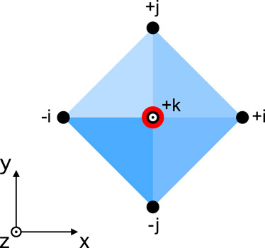
Figure 1. Basic single octahedron configuration and the labels employed for its corners (the $-k$ corner is not visible).

where $\mathbb{I}$ is the identity matrix in ${\mathbb{R}}^3$.

$\mathbf{F}=\left(\begin{array}{ccc}\hfill 1\hfill & \hfill 0\hfill & \hfill 0\hfill \\ \hfill 0\hfill & \hfill 1\hfill & \hfill 0\hfill \\ \hfill 0\hfill & \hfill 0\hfill & \hfill f\hfill \end{array}\right),(2)$

with $f$ being a positive number, and

$\mathbf{P}=\mathbf{L}\mathbf{G}\mathbf{R},(3)$

where

$\mathbf{L}=\left(\begin{array}{ccc}\hfill a^{\prime }\hfill & \hfill 0\hfill & \hfill 0\hfill \\ \hfill 0\hfill & \hfill b^{\prime }\hfill & \hfill 0\hfill \\ \hfill 0\hfill & \hfill 0\hfill & \hfill c^{\prime }\hfill \end{array}\right),(4)$

$\mathbf{G}=\left(\begin{array}{ccc}1& 0& 0\\ \cos \left({\gamma }^{\prime }\right)& \sin \left({\gamma }^{\prime }\right)& 0\\ \cos \left({\beta }^{\prime }\right)& \frac{\cos \left({\alpha }^{\prime }\right)-\cos \left({\beta }^{\prime }\right)\cos \left({\gamma }^{\prime }\right)}{\sin \left({\gamma }^{\prime }\right)}& \sqrt{1-{\cos }^2\left({\beta }^{\prime }\right)-{\left(\frac{\cos \left({\alpha }^{\prime }\right)-\cos \left({\beta }^{\prime }\right)\cos \left({\gamma }^{\prime }\right)}{\sin \left({\gamma }^{\prime }\right)}\right)}^2}\end{array}\right),(5)$

with $a^{\prime }$, $b^{\prime }$, and $c^{\prime }$ representing the arm lengths of the octahedron (not to be confused with lattice constants) and ${\alpha }^{\prime }$, ${\beta }^{\prime }$, and ${\gamma }^{\prime }$ representing the angles between the arms. If ${\alpha }^{\prime }={\beta }^{\prime }={\gamma }^{\prime }=$90°, the octahedron is orthogonal, indicating that its arm lengths are always perpendicular to each other. The matrix $\mathbf{R}={\mathbf{R}}^Z{\mathbf{R}}^X{\mathbf{R}}^Y$ is a general rotation in $SO(3)$, employing the covariant Tait–Bryan ${\mathbf{Y}}_{1={\varphi }_y}{\mathbf{X}}_{2={\varphi }_x}{\mathbf{Z}}_{3=\theta }$ convention (Berner, 2008; Roithmayr and Hodges, 2016), with the angles measured with respect to the reference system in Figure 1. Explicitly,

$\mathbf{R}=\left(\begin{array}{ccc}sin\left(\theta \right)sin\left({\varphi }_x\right)sin\left({\varphi }_y\right)+cos\left(\theta \right)cos\left({\varphi }_y\right)& sin\left(\theta \right)cos\left({\varphi }_x\right)& sin\left(\theta \right)sin\left({\varphi }_x\right)cos\left({\varphi }_y\right)-cos\left(\theta \right)sin\left({\varphi }_y\right)\\ cos\left(\theta \right)sin\left({\varphi }_x\right)sin\left({\varphi }_y\right)-sin\left(\theta \right)cos\left({\varphi }_y\right)& cos\left(\theta \right)cos\left({\varphi }_x\right)& cos\left(\theta \right)sin\left({\varphi }_x\right)cos\left({\varphi }_y\right)+sin\left(\theta \right)sin\left({\varphi }_y\right)\\ cos\left({\varphi }_x\right)sin\left({\varphi }_y\right)& -sin\left({\varphi }_x\right)& cos\left({\varphi }_x\right)cos\left({\varphi }_y\right)\end{array}\right),$

where we can recover the rotation angles from $\mathbf{R}$ via the following transformation:

$\theta =\arctan \left(\frac{R_{12}}{R_{22}}\right),(6)$

${\varphi }_x=\arcsin \left(-R_{32}\right),(7)$

${\varphi }_y=\arctan \left(\frac{R_{31}}{R_{33}}\right).(8)$

The parameter $f$ allows for distortion of an otherwise centrosymmetric octahedron along the apical direction, a situation commonly encountered in the outer layers of Ruddlesden–Popper phases, for example. More exotic non-centrosymmetric distortions are not included in the model, but they can be considered in the $\mathbf{F}$ matrix by using a more general definition than Equation 2. Furthermore,

$1_6={\left(\begin{array}{cccccc}\hfill 1\hfill & \hfill 1\hfill & \hfill 1\hfill & \hfill 1\hfill & \hfill 1\hfill & \hfill 1\hfill \end{array}\right)}^T,$

and $\mathbf{D}$ is a translation vector in ${\mathbb{R}}^3$. We define the nucleus of the octahedron as follows:

$\mathbf{A}=\left(\begin{array}{c}\hfill \mathbb{I}\hfill \\ \hfill -\mathbf{F}\hfill \end{array}\right)\mathbf{P},(9)$

so that the octahedron can be written as

$\mathbf{O}=\mathbf{A}+1_6\mathbf{D}.(10)$

An example showing the effect of varying the different parameters of a single octahedron is shown in Figure 2. Next, we define the octahedron sub-site operators:

$S^{+i}=\left(\begin{array}{cccccc}\hfill 1\hfill & \hfill 0\hfill & \hfill 0\hfill & \hfill 0\hfill & \hfill 0\hfill & \hfill 0\hfill \end{array}\right),$

$S^{+j}=\left(\begin{array}{cccccc}\hfill 0\hfill & \hfill 1\hfill & \hfill 0\hfill & \hfill 0\hfill & \hfill 0\hfill & \hfill 0\hfill \end{array}\right),$

$S^{+k}=\left(\begin{array}{cccccc}\hfill 0\hfill & \hfill 0\hfill & \hfill 1\hfill & \hfill 0\hfill & \hfill 0\hfill & \hfill 0\hfill \end{array}\right),$

$S^{-i}=\left(\begin{array}{cccccc}\hfill 0\hfill & \hfill 0\hfill & \hfill 0\hfill & \hfill 1\hfill & \hfill 0\hfill & \hfill 0\hfill \end{array}\right),$

$S^{-j}=\left(\begin{array}{cccccc}\hfill 0\hfill & \hfill 0\hfill & \hfill 0\hfill & \hfill 0\hfill & \hfill 1\hfill & \hfill 0\hfill \end{array}\right),$

$S^{-k}=\left(\begin{array}{cccccc}\hfill 0\hfill & \hfill 0\hfill & \hfill 0\hfill & \hfill 0\hfill & \hfill 0\hfill & \hfill 1\hfill \end{array}\right).$

Figure 2

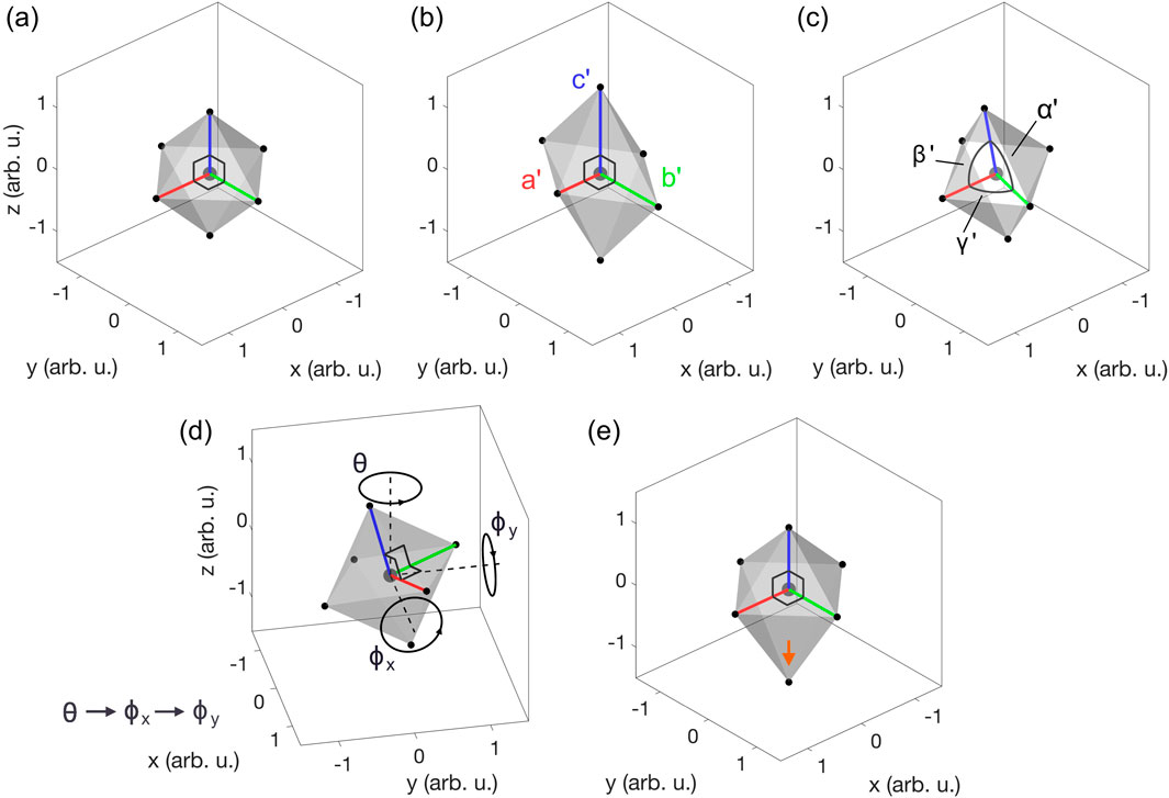
Figure 2. Parametrization of a single octahedron. (A) Regular, orthogonal octahedron of unitary arm length. (B) Non-regular, orthogonal octahedron with arm lengths $a^{\prime }=0.8$, $b^{\prime }=1.2$, and $c^{\prime }=1.4$. (C) Non-orthogonal octahedron with angles ${\alpha }^{\prime }=$101°, ${\beta }^{\prime }=$88°, and ${\gamma }^{\prime }=$76°. (D) Rotated, regular, orthogonal octahedron with rotation angles $\theta =$16.7°, ${\varphi }_x=$13.4°, and ${\varphi }_y=-$11.3°. The order of the rotations is specified. (E) Orthogonal octahedron with an apical distortion of $f=1.5$. The arrow indicates the displacement of the apical position.

When these operators act on an octahedron $\mathbf{O}$, they return the corresponding corner (see Figure 1). Then, it follows that

$\begin{array}{c}\hfill {\mathbf{O}}^{\pm n}=S^{\pm n}\mathbf{O}\\ \hfill =S^{\pm n}\mathbf{A}+\mathbf{D}\\ \hfill =S^{\pm n}\left(\begin{array}{c}\hfill \mathbb{I}\hfill \\ \hfill -\mathbf{F}\hfill \end{array}\right)\mathbf{P}+\mathbf{D}\\ \hfill =\pm \widehat{n}{f}^{\pm n}\mathbf{P}+\mathbf{D},\end{array}(11)$

where $n\in \{i,j,k\}$, $\widehat{n}$ is the corresponding canonical unit vector in ${\mathbb{R}}^3$, and $f^{\pm n}$ are all equal to 1, except for $f^{-k}=f$. The centroid of an octahedron is then given by

$\mathbf{C}=\frac{1}{6}{\displaystyle \sum _n}{\mathbf{O}}^n+{\mathbf{O}}^{-n}=\frac{\widehat{k}\left(1-f\right)\mathbf{P}}{6}+\mathbf{D}.(12)$

1.3 Extracting parameters from a single octahedron

To benefit from the parametrization given above in studying a particular system, we must first extract the octahedral information from its crystal structure. In other words, we want to build a set of relations that take the corners of an octahedron ($\mathbf{O}$-matrix) as input and determine its $\mathbf{F}$-, $\mathbf{L}$-, $\mathbf{G}$-, and $\mathbf{R}$-matrices. From Equation 1, we begin by splitting the known $\mathbf{O}$-matrix:

${\mathbf{O}}^{+}=\mathbf{P}+1_3\mathbf{D},$

${\mathbf{O}}^{-}=-\mathbf{F}\mathbf{P}+1_3\mathbf{D},$

where $1_3={\left(\begin{array}{ccc}\hfill 1\hfill & \hfill 1\hfill & \hfill 1\hfill \end{array}\right)}^T$. Then, we define ${\mathbf{O}}_g$ and ${\mathbf{W}}_g$ such that

${\mathbf{O}}_g=\frac{{\mathbf{O}}^{+}-{\mathbf{O}}^{-}}{2}=\left(\begin{array}{ccc}\hfill 1\hfill & \hfill 0\hfill & \hfill 0\hfill \\ \hfill 0\hfill & \hfill 1\hfill & \hfill 0\hfill \\ \hfill 0\hfill & \hfill 0\hfill & \hfill g\hfill \end{array}\right)\mathbf{L}\mathbf{G}\mathbf{R}={\mathbf{W}}_g\mathbf{R},(13)$

where $g=\frac{f+1}{2}$. However, ${\mathbf{O}}_g$ is simply the product of the lower triangular matrix ${\mathbf{W}}_g$ (see Equations 4, 5) and $\mathbf{R}\in SO(3)$. Therefore, we can apply the so-called $QR$ decomposition method on ${\mathbf{O}}_g^T$ (Gander, 1980) such that¹

$\begin{array}{c}\hfill {\mathbf{O}}_g^T={\mathbf{R}}^T{\mathbf{W}}_g^T\Rightarrow \\ \hfill {\mathbf{O}}_g={\mathbf{W}}_g\mathbf{R},\end{array}$

which is consistent with Equation 13. Thus, ${\mathbf{W}}_g$ and $\mathbf{R}$ are known, and we can directly extract the rotation angles from $\mathbf{R}$ using Equations 6–8. Moreover, ${\mathbf{W}}_g$ can be written as

${\mathbf{W}}_g=\left(\begin{array}{c}\hfill {\mathbf{W}}_1\hfill \\ \hfill {\mathbf{W}}_2\hfill \\ \hfill g{\mathbf{W}}_3,\hfill \end{array}\right),$

where each row is an octahedron arm vector, with the last one multiplied by the unknown factor $g$. From Equation 5, we can already extract the angles $\{{\alpha }^{\prime },{\beta }^{\prime },{\gamma }^{\prime }\}$ between the arm vectors using their dot products. Moreover, the arm lengths satisfy $a^{\prime }=\left|{\mathbf{W}}_1\right|$, $b^{\prime }=\left|{\mathbf{W}}_2\right|$, and $c^{\prime }g=\left|g{\mathbf{W}}_3\right|$, and thus, the only missing parameter is $f$ to determine $g$ and $c^{\prime }$. However, using Equation 12, we can show that

${\mathbf{O}}^{-}-1_3\mathbf{C}=\left(\begin{array}{ccc}\hfill -1\hfill & \hfill 0\hfill & \hfill \left(f-1\right)/6\hfill \\ \hfill 0\hfill & \hfill -1\hfill & \hfill \left(f-1\right)/6\hfill \\ \hfill 0\hfill & \hfill 0\hfill & \hfill -\left(5f+1\right)/6\hfill \end{array}\right)\mathbf{P},$

${\mathbf{O}}^{+}-1_3\mathbf{C}=\left(\begin{array}{ccc}\hfill 1\hfill & \hfill 0\hfill & \hfill \left(f-1\right)/6\hfill \\ \hfill 0\hfill & \hfill 1\hfill & \hfill \left(f-1\right)/6\hfill \\ \hfill 0\hfill & \hfill 0\hfill & \hfill \left(f+5\right)/6\hfill \end{array}\right)\mathbf{P},$

and define

${\mathbf{O}}_c=\left({\mathbf{O}}^{-}-1_3\mathbf{C}\right){\left({\mathbf{O}}^{+}-1_3\mathbf{C}\right)}^{-1}=\left(\begin{array}{ccc}\hfill -1\hfill & \hfill 0\hfill & \hfill 2\left(f-1\right)/\left(f+5\right)\hfill \\ \hfill 0\hfill & \hfill -1\hfill & \hfill 2\left(f-1\right)/\left(f+5\right)\hfill \\ \hfill 0\hfill & \hfill 0\hfill & \hfill -\left(5f+1\right)/\left(f+5\right)\hfill \end{array}\right).$

Thus,

$f=-\frac{5{\mathbf{O}}_c^{13}+2}{{\mathbf{O}}_c^{13}-2}=-\frac{5{\mathbf{O}}_c^{23}+2}{{\mathbf{O}}_c^{23}-2}=-\frac{5{\mathbf{O}}_c^{33}+1}{{\mathbf{O}}_c^{33}+5}.(14)$

Therefore, because the centroid $\mathbf{C}$ can be directly calculated from the $\mathbf{O}$-matrix, we have determined all the octahedron parameters. The definition of $f$ is over-determined in Equation 14. Thus, if the three different ways of calculating $f$ are not all consistent, the $\mathbf{O}$-matrix under consideration is beyond the description provided by the model in Equation 1. Finally, we define the off-centering vector as the difference between the position $\mathbf{Q}$ of the caged atom in the crystal structure and the centroid of the octahedron given by Equation 12:

$\mathbf{d}=\mathbf{Q}-\mathbf{C},$

which is non-zero in ferroelectric materials, even for centrosymmetric octahedra, for example.

1.4 The 4-octahedra general case

We now create a system of four octahedra connected through their corners, as shown in Figure 3, such that the individual octahedra are free to rotate or distort but remain linked at all times. We call this system 4-octahedra, which we then use as a building block to form a lattice. In doing so, we determine all possible bond lengths, bond angles, and octahedral rotations within the 4-octahedra that are compatible with up to four inequivalent sites. According to Equation 10, we can express an individual octahedron as follows:

${\mathbf{O}}_s=\left({\mathbf{A}}_s^{\prime }+1_6{\mathbf{D}}_s^{\prime }\right){\mathbf{R}}_f={\mathbf{A}}_s+1_6{\mathbf{D}}_s,$

Figure 3

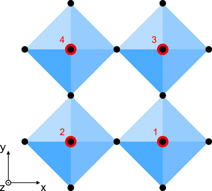
Figure 3. Basic 4-octahedral configuration. The octahedral numbering convention is indicated.

where $s\in \{\mathrm{1,2,3,4}\}$, and we have introduced the rotational freedom matrix ${\mathbf{R}}_f\in SO(3)$, a rigid rotation common to the four octahedra that we can fix later without loss of generality. The primed notation in the first identity refers to the single octahedron parameters before addressing the system’s rotational freedom. That is, ${\mathbf{A}}_s={\mathbf{A}}_s^{\prime }{\mathbf{R}}_f$ and ${\mathbf{D}}_s={\mathbf{D}}_s^{\prime }{\mathbf{R}}_f$, which show that the system rotation affects the nucleus ${\mathbf{A}}_s^{\prime }$ of the individual octahedra and their displacements ${\mathbf{D}}_s^{\prime }$. Nevertheless, from Equations 3, 9 and the properties of $SO(3)$, we see that ${\mathbf{R}}_f$ is absorbed by the particular single octahedron $\mathbf{R}$-matrix such that ${\mathbf{L}}_s={\mathbf{L}}_s^{\prime }$, ${\mathbf{G}}_s={\mathbf{G}}_s^{\prime }$, and ${\mathbf{R}}_s={\mathbf{R}}_s^{\prime }{\mathbf{R}}_f$. Thus, the rigid rotation does not affect the internal structure of the octahedra encoded in the $\mathbf{L}$- and $\mathbf{G}$-matrices, and we can write

${\mathbf{P}}_s={\mathbf{P}}_s^{\prime }{\mathbf{R}}_f={\mathbf{L}}_s{\mathbf{G}}_s{\mathbf{R}}_s^{\prime }{\mathbf{R}}_f.(15)$

Now, the conditions for having the four octahedra connected through their corners, as shown in Figure 3, are as follows:

${\mathbf{O}}_1^{-i}={\mathbf{O}}_2^{+i},(16)$

${\mathbf{O}}_1^{+j}={\mathbf{O}}_3^{-j},(17)$

${\mathbf{O}}_2^{+j}={\mathbf{O}}_4^{-j},(18)$

${\mathbf{O}}_3^{-i}={\mathbf{O}}_4^{+i}.(19)$

From these and Equation 11, we obtain the following set of equations:

$-\widehat{i}{\mathbf{P}}_1+{\mathbf{D}}_1=\widehat{i}{\mathbf{P}}_2+{\mathbf{D}}_2,(20)$

$\widehat{j}{\mathbf{P}}_1+{\mathbf{D}}_1=-\widehat{j}{\mathbf{P}}_3+{\mathbf{D}}_3,(21)$

$\widehat{j}{\mathbf{P}}_2+{\mathbf{D}}_2=-\widehat{j}{\mathbf{P}}_4+{\mathbf{D}}_4,(22)$

$-\widehat{i}{\mathbf{P}}_3+{\mathbf{D}}_3=\widehat{i}{\mathbf{P}}_4+{\mathbf{D}}_4,(23)$

which we rearrange to get the following relationships between the octahedral displacements:

$\left(\widehat{i}-\widehat{j}\right)\left({\mathbf{P}}_1+{\mathbf{P}}_2+{\mathbf{P}}_3+{\mathbf{P}}_4\right)+2\left({\mathbf{D}}_4-{\mathbf{D}}_1\right)=0,(24)$

$\left(\widehat{i}+\widehat{j}\right)\left({\mathbf{P}}_1+{\mathbf{P}}_2+{\mathbf{P}}_3+{\mathbf{P}}_4\right)+2\left({\mathbf{D}}_2-{\mathbf{D}}_3\right)=0,(25)$

and a displacement-independent structural equation, which provides a necessary and sufficient condition for the octahedra to be linkable (see Figures 4A, B):

$\left(\widehat{i}+\widehat{j}\right)\left({\mathbf{P}}_1-{\mathbf{P}}_4\right)+\left(\widehat{i}-\widehat{j}\right)\left({\mathbf{P}}_2-{\mathbf{P}}_3\right)=0.(26)$

Figure 4

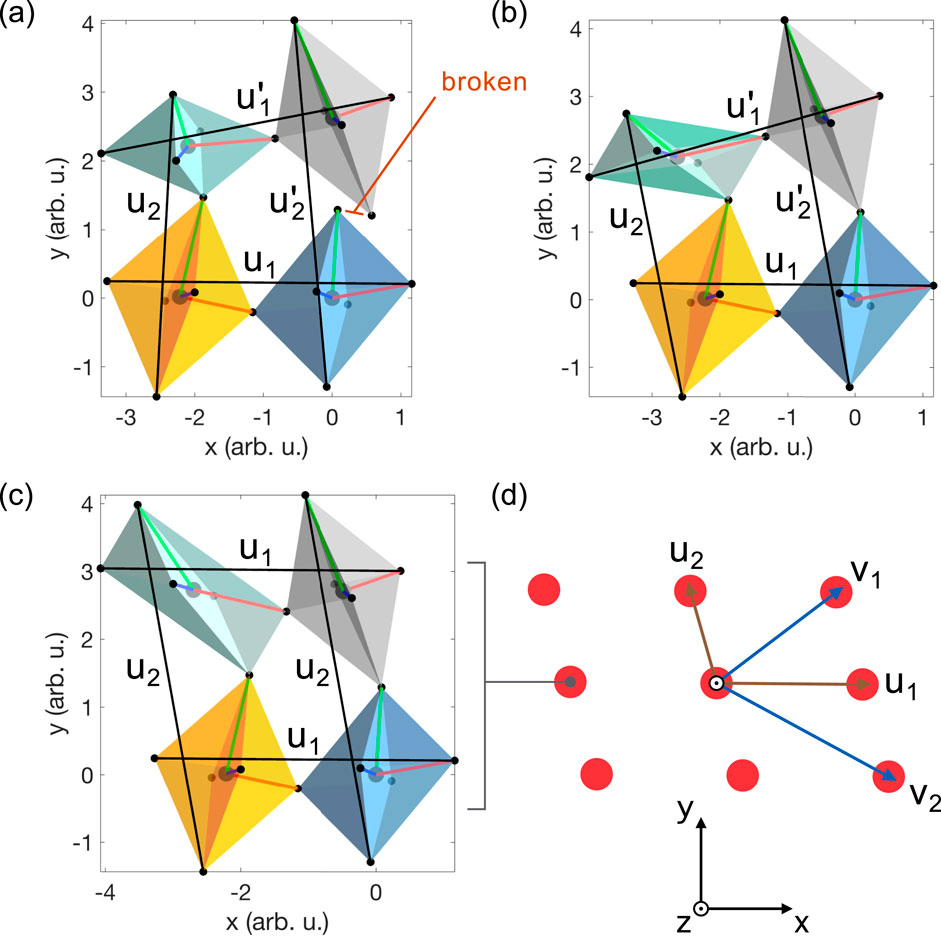
Figure 4. Formation of the 4-octahedral lattice. (A) 4-Octahedral model that does not satisfy Equation 26, showing a broken link and the impossibility to form a lattice. (B) 4-Octahedral model that does satisfy Equation 26, but not Equations 37, 38, showing octahedral linking incompatible with lattice formation. (C) 4-Octahedra satisfying Equations 37, 38 and exhibiting octahedral linking compatible with lattice formation. (D) The primitive and conventional lattice vectors of the 4-octahedral lattice formed by the 4-octahedra in (C), where each point represents a 4-octahedral unit. The lattice is monoclinic with $C_1\ne 0$ and $C_2\ne 0$.

Furthermore, without loss of generality, we fix the translational freedom of the 4-octahedra such that

${\mathbf{D}}_1+{\mathbf{D}}_2+{\mathbf{D}}_3+{\mathbf{D}}_4=\mathbf{0},(27)$

and we define a site-equivalency operator between two octahedra as follows:

$\mathcal{E}\left({\mathbf{O}}_i,{\mathbf{O}}_j\right)=\left({\mathbf{O}}_i-1_6{\mathbf{D}}_i\right)-\left({\mathbf{O}}_j-1_6{\mathbf{D}}_j\right)={\mathbf{A}}_i-{\mathbf{A}}_j.$

Therefore, two sites are equivalent if $\mathcal{E}({\mathbf{O}}_i,{\mathbf{O}}_j)=0$, that is, if ${\mathbf{A}}_i={\mathbf{A}}_j$. We see that our general model mentioned above supports up to four inequivalent sites. The previous equations are quite general and guarantee that the 4-octahedra will remain connected through their corners; however, they do not imply that the 4-octahedra is compatible with forming a lattice (see Figure 4B).

1.5 The 4-Octahedra lattice

In order for the 4-octahedra to form a two-dimensional lattice, we must impose periodic boundary conditions such that the bottom (left) corners in Figure 3 connect with the top (right) corners modulo two linearly independent vectors $\{{\mathbf{u}}_1,{\mathbf{u}}_2\}$; that is, we want to map any point of the 4-octahedra to the same point in another unit cell. This implies that

$\widehat{i}{\mathbf{P}}_1+{\mathbf{D}}_1=-\widehat{i}{\mathbf{P}}_2+{\mathbf{D}}_2+{\mathbf{u}}_1,(28)$

$\widehat{i}{\mathbf{P}}_3+{\mathbf{D}}_3=-\widehat{i}{\mathbf{P}}_4+{\mathbf{D}}_4+{\mathbf{u}}_1,(29)$

$\widehat{j}{\mathbf{P}}_3+{\mathbf{D}}_3=-\widehat{j}{\mathbf{P}}_1+{\mathbf{D}}_1+{\mathbf{u}}_2,(30)$

$\widehat{j}{\mathbf{P}}_4+{\mathbf{D}}_4=-\widehat{j}{\mathbf{P}}_2+{\mathbf{D}}_2+{\mathbf{u}}_2,(31)$

which are clearly not satisfied in Figure 4B, where there is no unique $\{{\mathbf{u}}_1,{\mathbf{u}}_2\}$ that connects the corners. If we now define

$\mathbf{V}={\mathbf{D}}_1-{\mathbf{D}}_2-{\mathbf{D}}_3+{\mathbf{D}}_4(32)$

and eliminate ${\mathbf{u}}_1$ and ${\mathbf{u}}_2$ in the equations above, we obtain

$\widehat{i}\left({\mathbf{P}}_1+{\mathbf{P}}_2-{\mathbf{P}}_3-{\mathbf{P}}_4\right)=-\mathbf{V},(33)$

$\widehat{j}\left({\mathbf{P}}_1-{\mathbf{P}}_2+{\mathbf{P}}_3-{\mathbf{P}}_4\right)=\mathbf{V}.(34)$

Moreover, combining Equations 20, 23 and Equations 21, 22 yields

$\widehat{i}\left({\mathbf{P}}_1+{\mathbf{P}}_2-{\mathbf{P}}_3-{\mathbf{P}}_4\right)=\mathbf{V},(35)$

$\widehat{j}\left({\mathbf{P}}_1-{\mathbf{P}}_2+{\mathbf{P}}_3-{\mathbf{P}}_4\right)=-\mathbf{V}.(36)$

Equations 33–36 imply that $\mathbf{V}=0$ and

$\widehat{i}\left({\mathbf{P}}_1+{\mathbf{P}}_2-{\mathbf{P}}_3-{\mathbf{P}}_4\right)=0,(37)$

$\widehat{j}\left({\mathbf{P}}_1-{\mathbf{P}}_2+{\mathbf{P}}_3-{\mathbf{P}}_4\right)=0,(38)$

which are displacement-independent structural conditions for the 4-octahedra to form a lattice. Moreover, the sum of the last two identities yields Equation 26. Thus, if satisfied, the lattice equations automatically imply octahedral linking. Furthermore, from Equation 32,

${\mathbf{D}}_1+{\mathbf{D}}_4={\mathbf{D}}_2+{\mathbf{D}}_3.$

Therefore, using the condition in Equation 27, we obtain

${\mathbf{D}}_1=-{\mathbf{D}}_4,(39)$

${\mathbf{D}}_2=-{\mathbf{D}}_3.(40)$

Thus, we see that the octahedral displacements lie in the same plane. Equations 37, 38 hold immediately in monopartite $({\mathbf{P}}_1={\mathbf{P}}_2={\mathbf{P}}_3={\mathbf{P}}_4)$ and bipartite (${\mathbf{P}}_1={\mathbf{P}}_4$ and ${\mathbf{P}}_2={\mathbf{P}}_3$) lattices, which means that we can always take one or two random octahedra (regardless of their form or orientation) and connect their corners to form a lattice. However, if we take four random octahedra and link the second to the first, the third to the second, and the fourth to the third, it might well be that the fourth octahedron will not be connected to the first (see Figure 4A) or that the octahedra get all connected but cannot form a lattice (see Figure 4B). Thus, with four inequivalent sites, Equations 37, 38 dictate how to select the octahedra so that they are guaranteed to connect and form a lattice. An example of this is illustrated in Figure 4C, showing the uniqueness of the lattice vectors and the octahedral linking.

Substituting Equations 39, 40 into Equations 24, 25 yields

${\mathbf{D}}_1=\frac{\left(\widehat{i}-\widehat{j}\right)}{4}\bar{\mathbf{P}},(41)$

${\mathbf{D}}_3=\frac{\left(\widehat{i}+\widehat{j}\right)}{4}\bar{\mathbf{P}},(42)$

where we have defined the $\bar{\mathbf{P}}$-matrix of the system²:

$\bar{\mathbf{P}}={\mathbf{P}}_1+{\mathbf{P}}_2+{\mathbf{P}}_3+{\mathbf{P}}_4.(43)$

Moreover, adding Equations 28, 29 and Equations 30, 31 and then using Equations 39, 40 and Equations 41, 42 yield

${\mathbf{u}}_1=2\left({\mathbf{D}}_1+{\mathbf{D}}_3\right)=\widehat{i}\bar{\mathbf{P}},(44)$

${\mathbf{u}}_2=2\left({\mathbf{D}}_3-{\mathbf{D}}_1\right)=\widehat{j}\bar{\mathbf{P}},(45)$

which define the primitive lattice vectors of the system as a function of the octahedral displacements or the $\bar{\mathbf{P}}$-matrix alone. Finally, we define the conventional lattice vectors

${\mathbf{v}}_1={\mathbf{u}}_1+{\mathbf{u}}_2=\left(\widehat{i}+\widehat{j}\right)\bar{\mathbf{P}},(46)$

${\mathbf{v}}_2={\mathbf{u}}_1-{\mathbf{u}}_2=\left(\widehat{i}-\widehat{j}\right)\bar{\mathbf{P}},(47)$

which run diagonally across the 4-octahedra lattice (see Figure 4D).

1.6 Relationship between the lattice and the 4-octahedra configuration

In this section, we establish a set of geometric relations that link the global properties of the lattice, such as the vector length and the projections between them, to the specific octahedral geometry and rotation angles encoded in the $\bar{\mathbf{P}}$-matrix. We start by evaluating the projection between the conventional vectors:

$\begin{array}{c}\hfill {\mathbf{v}}_1\cdot {\mathbf{v}}_2=\left(\widehat{i}+\widehat{j}\right)\bar{\mathbf{P}}\cdot \left(\widehat{i}-\widehat{j}\right)\bar{\mathbf{P}}=\left(\widehat{i}+\widehat{j}\right)\bar{\mathbf{P}}{\bar{\mathbf{P}}}^T{\left(\widehat{i}-\widehat{j}\right)}^T,\end{array}(48)$

and the projection between the primitive vectors:

$\begin{array}{c}\hfill {\mathbf{u}}_1\cdot {\mathbf{u}}_2=\widehat{i}\bar{\mathbf{P}}\cdot \widehat{j}\bar{\mathbf{P}}=\widehat{i}\bar{\mathbf{P}}{\bar{\mathbf{P}}}^T{\widehat{j}}^T.\end{array}(49)$

Now, we evaluate the length difference between the conventional vectors:

$\begin{array}{c}\hfill {\mathbf{v}}_1\cdot {\mathbf{v}}_1-{\mathbf{v}}_2\cdot {\mathbf{v}}_2=\left(\widehat{i}+\widehat{j}\right)\bar{\mathbf{P}}{\bar{\mathbf{P}}}^T{\left(\widehat{i}+\widehat{j}\right)}^T-\left(\widehat{i}-\widehat{j}\right)\bar{\mathbf{P}}{\bar{\mathbf{P}}}^T{\left(\widehat{i}-\widehat{j}\right)}^T\\ \hfill =2\widehat{j}\bar{\mathbf{P}}{\bar{\mathbf{P}}}^T{\widehat{i}}^T+2\widehat{i}\bar{\mathbf{P}}{\bar{\mathbf{P}}}^T{\widehat{j}}^T=4\widehat{i}\bar{\mathbf{P}}{\bar{\mathbf{P}}}^T{\widehat{j}}^T,\end{array}(50)$

and the length difference between the primitive vectors:

$\begin{array}{c}\hfill {\mathbf{u}}_1\cdot {\mathbf{u}}_1-{\mathbf{u}}_2\cdot {\mathbf{u}}_2=\widehat{i}\bar{\mathbf{P}}{\bar{\mathbf{P}}}^T{\widehat{i}}^T-\widehat{j}\bar{\mathbf{P}}{\bar{\mathbf{P}}}^T{\widehat{j}}^T\\ \hfill =\widehat{i}\bar{\mathbf{P}}{\bar{\mathbf{P}}}^T{\widehat{i}}^T-\widehat{i}\bar{\mathbf{P}}{\bar{\mathbf{P}}}^T{\widehat{j}}^T-\widehat{j}\bar{\mathbf{P}}{\bar{\mathbf{P}}}^T{\widehat{j}}^T+\widehat{j}\bar{\mathbf{P}}{\bar{\mathbf{P}}}^T{\widehat{i}}^T=\left(\widehat{i}+\widehat{j}\right)\bar{\mathbf{P}}{\bar{\mathbf{P}}}^T{\left(\widehat{i}-\widehat{j}\right)}^T.\end{array}(51)$

1.7 Main theorem of the 4-octahedra lattice

From Equations 48–51, we have shown that

${\left|{\mathbf{u}}_1\right|}^2-{\left|{\mathbf{u}}_2\right|}^2={\mathbf{v}}_1\cdot {\mathbf{v}}_2=C_1,$

$\frac{{\left|{\mathbf{v}}_1\right|}^2-{\left|{\mathbf{v}}_2\right|}^2}{4}={\mathbf{u}}_1\cdot {\mathbf{u}}_2=C_2,$

where we define the geometric scalar fields:

$C_1=\left(\widehat{i}+\widehat{j}\right)\bar{\mathbf{P}}{\bar{\mathbf{P}}}^T{\left(\widehat{i}-\widehat{j}\right)}^T,(52)$

$C_2=\widehat{i}\bar{\mathbf{P}}{\bar{\mathbf{P}}}^T{\widehat{j}}^T.(53)$

Thus, we see that

$\left|{\mathbf{u}}_1\right|=\left|{\mathbf{u}}_2\right|⟺{\mathbf{v}}_1\cdot {\mathbf{v}}_2=0⟺C_1=0,$

$\left|{\mathbf{v}}_1\right|=\left|{\mathbf{v}}_2\right|⟺{\mathbf{u}}_1\cdot {\mathbf{u}}_2=0⟺C_2=0,$

which we refer to as conditions (1) and (2), respectively. It follows that

$•$ If conditions (1) and (2) are satisfied, the system is tetragonal (T).

$•$ If only condition (1) holds, the system is rectangular orthorhombic (R. O.).

$•$ If only condition (2) holds, the system is centered orthorhombic (C. O.).

$•$ If none of the conditions are satisfied, the system is monoclinic (M).

Therefore, we can map the octahedral configuration to the lattice geometry using only two parameters $C_1$ and $C_2$. The example in Figure 4D shows the most general case of a monoclinic lattice.

1.8 Addressing the system rotational freedom

Just as we fixed the translational freedom of the 4-octahedra, we can (without loss of generality) choose the displacements of the octahedra to lie entirely within the $xy$-plane:

$\begin{array}{c}\hfill {\mathbf{D}}_1{\widehat{k}}^T={\mathbf{D}}_4{\widehat{k}}^T\Rightarrow \\ \hfill {\mathbf{D}}_1{\widehat{k}}^T=0\Rightarrow \\ \hfill \left(\widehat{i}-\widehat{j}\right)\bar{\mathbf{P}}{\widehat{k}}^T=0,\end{array}(54)$

$\begin{array}{c}\hfill {\mathbf{D}}_2{\widehat{k}}^T={\mathbf{D}}_3{\widehat{k}}^T\Rightarrow \\ \hfill {\mathbf{D}}_3{\widehat{k}}^T=0\Rightarrow \\ \hfill \left(\widehat{i}+\widehat{j}\right)\bar{\mathbf{P}}{\widehat{k}}^T=0.\end{array}(55)$

Furthermore, to fix the in-plane rotational freedom, we can set the displacements 1 and 2 to lie along the $x$-axis:

$\begin{array}{c}\hfill {\mathbf{D}}_1{\widehat{j}}^T={\mathbf{D}}_2{\widehat{j}}^T\Rightarrow \\ \hfill \left(\widehat{i}-\widehat{j}\right)\bar{\mathbf{P}}{\widehat{j}}^T=-\left(\widehat{i}+\widehat{j}\right)\bar{\mathbf{P}}{\widehat{j}}^T\Rightarrow \\ \hfill \widehat{i}\bar{\mathbf{P}}{\widehat{j}}^T=0.\end{array}(56)$

Thus, rearranging Equations 54–56, we obtain

$\widehat{i}\bar{\mathbf{P}}{\widehat{j}}^T={\bar{\mathbf{P}}}_{12}=0,(57)$

$\widehat{i}\bar{\mathbf{P}}{\widehat{k}}^T={\bar{\mathbf{P}}}_{13}=0,(58)$

$\widehat{j}\bar{\mathbf{P}}{\widehat{k}}^T={\bar{\mathbf{P}}}_{23}=0,(59)$

which means that we must choose $\bar{\mathbf{P}}$ to be lower-triangular. If our initial ${\bar{\mathbf{P}}}^{\prime }$ matrix in Equation 43 is not lower-triangular, we can triangularize it by applying the $QR$ decomposition method on ${\bar{\mathbf{P}}}^{\prime T}$ such that

$\begin{array}{c}\hfill {\bar{\mathbf{P}}}^{\prime T}={\mathbf{R}}_f{\bar{\mathbf{P}}}_{ut}^{\prime }\Rightarrow \\ \hfill {\bar{\mathbf{P}}}^{\prime }={\bar{\mathbf{P}}}_{lt}^{\prime }{\mathbf{R}}_f^T\Rightarrow \\ \hfill {\bar{\mathbf{P}}}_{lt}^{\prime }={\bar{\mathbf{P}}}^{\prime }{\mathbf{R}}_f=\bar{\mathbf{P}},\end{array}(60)$

where ${\mathbf{R}}_f$ is the rotational freedom matrix (the rotation matrix that aligns the 4-octahedra with the global rotational configuration chosen in Equations 57–59) and ${\bar{\mathbf{P}}}_{ut}^{\prime }$ is the upper-triangularization of ${\bar{\mathbf{P}}}^{\prime T}$. Both ${\mathbf{R}}_f$ and ${\bar{\mathbf{P}}}_{ut}^{\prime }$ are obtained using the $QR$ decomposition method. Once these are known, from Equation 60, we directly obtain the lower triangular $\bar{\mathbf{P}}$-matrix as ${\bar{\mathbf{P}}}_{lt}^{\prime }$, which is the lower-triangularization of ${\bar{\mathbf{P}}}^{\prime }$. Note that once ${\bar{\mathbf{P}}}^{\prime }$ is lower triangular (i.e., ${\bar{\mathbf{P}}}^{\prime }={\bar{\mathbf{P}}}_{lt}^{\prime }$), it follows that ${\mathbf{R}}_f=\mathbb{I}$, and the system no longer has rotational freedom.

1.9 Toward three-dimensions and $N>4$ sites

A generalization that would allow the description of many more octahedral configurations implies extending the model to three dimensions and scaling it to support $N>4$ inequivalent sites, especially relevant for systems with large unit cells and displaying complex octahedral arrangements beyond Glazer notation (Glazer, 1972; Grosso and Spaldin, 2021). In short, defining a three-dimensional $N$-octahedral model is possible. By analogy with the derivation of the 4-octahedra model in Sections 1.4–1.8, the procedure is as follows:

$•$ Define linking equations between $N$ octahedra to form a $N$-octahedra unit (see Equations 16–19). In three dimensions, linking conditions must also exist between $k$-corners.

$•$ Find displacement-independent structural equations for the octahedra to be linkable (see Equation 26).

$•$ Fix the translational freedom of the $N$-octahedra unit (see Equation 27).

$•$ Define periodic boundary conditions on the $N$-octahedra unit (see Equations 28–31). In three dimensions, periodic boundary conditions also exist between $k$-corners, and three primitive lattice vectors must be found.

$•$ Find displacement-independent structural conditions for the $N$-octahedra to form a lattice (see Equations 37, 38).

$•$ Solve the octahedral displacements (see Equations 39–42) and the lattice vectors (see Equations 44–47) in terms of the $\bar{\mathbf{P}}$-matrix of the system (see Equation 43):

$\bar{\mathbf{P}}={\displaystyle \sum _{i=1}^N}{\mathbf{P}}_i.$

$•$ In three dimensions, follow Sections 1.6, 1.7 to generalize the main theorem of the 4-octahedra using the relationships between the three lattice vectors and the $\bar{\mathbf{P}}$-matrix.

$•$ Following Section 1.8, address the global rotational freedom of the $N$-octahedra lattice.

The biggest drawback of this process is manipulating a large number of equations; however, the high level of symmetry displayed by the relationships suggests that there may be ways to automatize the algorithm, possibly using system matrices and other elements from linear algebra.

1.10 4-Octahedra two-site bipartite model

The model is chosen as a compromise between the generality afforded by multiple inequivalent sites while balancing the computational efficiency and analytical tractability; therefore, we now focus on the case where there are two inequivalent sites forming a bipartite lattice (checkerboard pattern), similar to the surface layer of ${\mathrm{S}\mathrm{r}}_2$RuO₄ (Morales et al., 2023) and also relevant for real distortions in many other systems. Thus, we impose the following symmetries to the 4-octahedra:

${\mathbf{A}}_1={\mathbf{A}}_4={\mathbf{A}}_A,$

${\mathbf{A}}_2={\mathbf{A}}_3={\mathbf{A}}_B.$

That is, sites 1 and 4 and sites 2 and 3 are equivalent, respectively, such that ${\mathbf{P}}_1={\mathbf{P}}_4={\mathbf{P}}_A$ and ${\mathbf{P}}_2={\mathbf{P}}_3={\mathbf{P}}_B$.³ Under these considerations, $\bar{\mathbf{P}}=2({\bar{\mathbf{P}}}_A+{\bar{\mathbf{P}}}_B)$, but we can define $\bar{\mathbf{P}}\to 2\bar{\mathbf{P}}$ for simplicity such that

$\bar{\mathbf{P}}={\mathbf{P}}_A+{\mathbf{P}}_B,(61)$

${\mathbf{D}}_1=\frac{\left(\widehat{i}-\widehat{j}\right)}{2}\bar{\mathbf{P}},$

${\mathbf{D}}_3=\frac{\left(\widehat{i}+\widehat{j}\right)}{2}\bar{\mathbf{P}},$

${\mathbf{u}}_1={\mathbf{D}}_1+{\mathbf{D}}_3=\widehat{i}\bar{\mathbf{P}},(62)$

${\mathbf{u}}_2={\mathbf{D}}_3-{\mathbf{D}}_1=\widehat{j}\bar{\mathbf{P}},(63)$

${\mathbf{v}}_1=\left(\widehat{i}+\widehat{j}\right)\bar{\mathbf{P}},$

${\mathbf{v}}_2=\left(\widehat{i}-\widehat{j}\right)\bar{\mathbf{P}},$

where we used the relevant equations from Section 1.5 and considered ${\mathbf{u}}_1\to 2{\mathbf{u}}_1$, ${\mathbf{u}}_2\to 2{\mathbf{u}}_2$, ${\mathbf{v}}_1\to 2{\mathbf{v}}_1$, and ${\mathbf{v}}_2\to 2{\mathbf{v}}_2$ to account for the reduction in the primitive unit cell. The vectors $\{{\mathbf{v}}_1,{\mathbf{v}}_2\}$ are now primitive lattice vectors, while $\{{\mathbf{u}}_1,{\mathbf{u}}_2\}$ are the so-called tetragonal vectors⁴. However, the main theorem of the 4-octahedra lattice still holds because these vectors exhibit the same dependence on the $\bar{\mathbf{P}}$-matrix as in the four-site general case. An example of a general bipartite model generated using the relationships above is shown in Figure 5, where the new vectors are indicated.

Figure 5

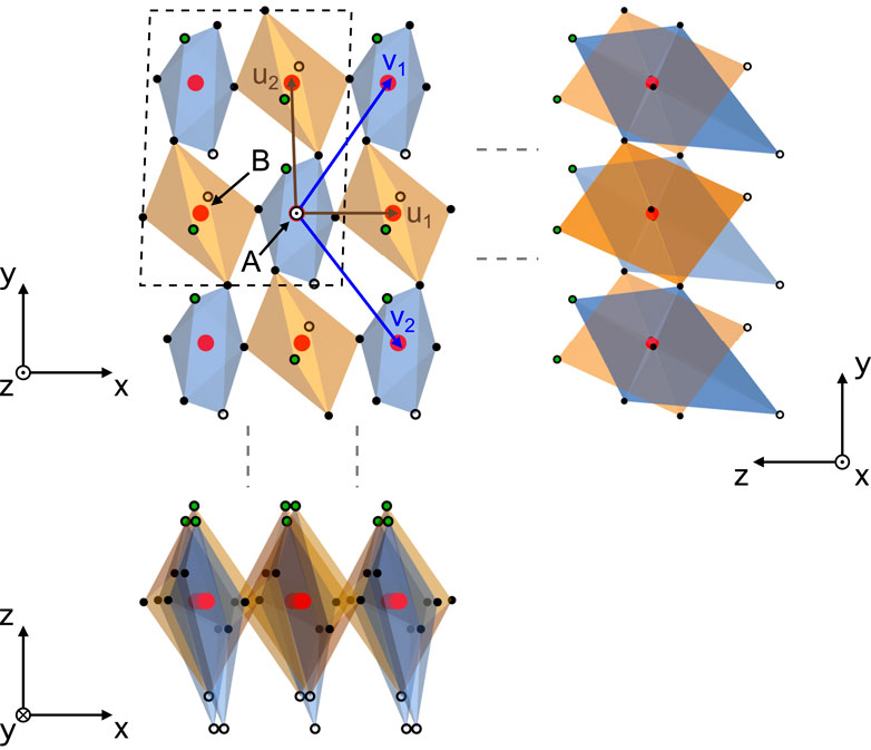
Figure 5. Bipartite model in a monoclinic configuration observed from different projections, where the 4-octahedra is enclosed by the dashed box. The arm lengths are $(a_A^{\prime }=0.8,b_A^{\prime }=1.4,c_A^{\prime }=1.9)$ and $(a_B^{\prime }=1.2,b_B^{\prime }=1.7,c_B^{\prime }=2)$, the angles between the arms are $({\alpha }_A^{\prime }=89°,{\beta }_A^{\prime }=101°,{\gamma }_A^{\prime }=76°)$ and $({\alpha }_B^{\prime }=78°,{\beta }_B^{\prime }=94°,{\gamma }_B^{\prime }=105°)$, the rotation angles are $({\theta }_A=-6.6°,{\varphi }_A^x=-24.4°,{\varphi }_A^y=4.2°)$ and $({\theta }_B=4.3°,{\varphi }_B^x=20.9°,{\varphi }_B^y=0.5°)$, and the apical distortions are set to $f_A=1.6$ and $f_B=1$. The top (bottom) apical corners are shown with green-filled (empty) open circles.

1.11 The 4-Octahedra model made accessible

The bipartite 4-octahedra model has been coded into MATLAB functions that facilitate its use and visualization (T. M. Inc, 2022). In this section, we review some examples that test the main function called Octahedron_algorithm.m, which is well commented and serves as a tutorial in combination with this text. The function takes as input the octahedral parameters at sites A and B and outputs the relevant system matrices and a three-dimensional visualization of the octahedral configuration. The simplest possible case is running the command:

Octahedron_algorithm([1 1 1 90 90 90 0 0 0 1],[1 1 1 90 90 90 0 0 0 1]);

in the MATLAB command window, which constructs a system of equivalent, undistorted, unrotated octahedra with arm lengths equal to unity. The first (second) array of numbers contains the octahedral parameters at site A (site B), with the following ordering:

[a’ b’ c’ alpha’ beta’ gamma’ theta phi_x phi_y f].

The function also accepts several optional arguments (documented in the code) that allow the manipulation of different visual elements of the system, such as colors, unit-cell drawings, and lattice extent. The basic example above is illustrated in Figure 6A, along with other octahedral configurations that the reader is encouraged to test. Figure 6B shows the formation of the stereotypical breathing mode by alternating the octahedral arm lengths between the sites. Figure 6C shows an example of in-plane bipartite rotation, encountered in the surface layer of Sr₂RuO₄ and the bulk of Sr₃Ru₂O₇ (Morales et al., 2023). Figures 6D, E illustrate how octahedral non-orthogonality alone may lead to different types of lattices. Finally, Figure 6F shows combined octahedral distortions and rotations that lead to an intricate configuration.

Figure 6

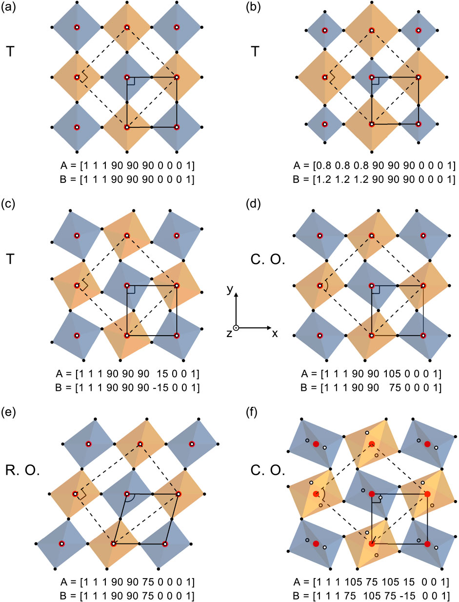
Figure 6. Examples of octahedral configurations built using the 4-octahedral parametrization. In each case, the arrays A and B are the input parameters of the Octahedron_algorithm.m function. The type of lattice is indicated, where the tetragonal cell is drawn using a black line and the primitive unit cell is shown with a dashed line. The top (bottom) apical corners are shown with white-filled (empty) open circles. (A) Basic 4-Octahedra configuration. (B) A simple octahedral breathing mode. (C) An example of in-plane bipartite rotation. (D,E) Octahedral non-orthogonality leading the formation of centered orthorhombic and rectangular orthorhombic lattices, respectively. (F) Complex octahedral configuration from combined in-plane rotation and non-orthogonal distortions.

1.12 A real example

The parametrization developed so far is quite general and can be employed to describe much more complicated geometries than the examples provided above (see Figure 5). More intuitively, we can test it on systems with a highly symmetric octahedral configuration, such as perovskites. Figure 7 shows contiguous planes of corner-sharing ${\mathrm{R}\mathrm{u}\mathrm{O}}_6$ octahedra extracted from ${\mathrm{S}\mathrm{r}\mathrm{R}\mathrm{u}\mathrm{O}}_3$. The planes are perpendicular to the $c$-axis, and the whole crystal in Figure 7A is recovered by alternating distinct A and B planes along the $z$-direction. If we apply the procedure described in Section 1.3 to the octahedra in each plane, we find that ${\mathrm{S}\mathrm{r}\mathrm{R}\mathrm{u}\mathrm{O}}_3$ is compatible with the 4-octahedra parametrization such that each plane forms a bipartite lattice, indicating that the crystal is made up of four inequivalent sites. Naturally, the obtained octahedral parameters carry the particular symmetries of the system. For example, the arm lengths in each plane satisfy $(a_A^{\prime }=b_B^{\prime },b_A^{\prime }=a_B^{\prime },\mathrm{a}\mathrm{n}\mathrm{d}{c}_A^{\prime }=c_B^{\prime })$ and the angles between the arms follow $({\alpha }_A^{\prime }={\beta }_B^{\prime },{\beta }_A^{\prime }={\alpha }_A^{\prime },\mathrm{a}\mathrm{n}\mathrm{d}{\gamma }_A^{\prime }={\gamma }_B^{\prime })$.

Figure 7

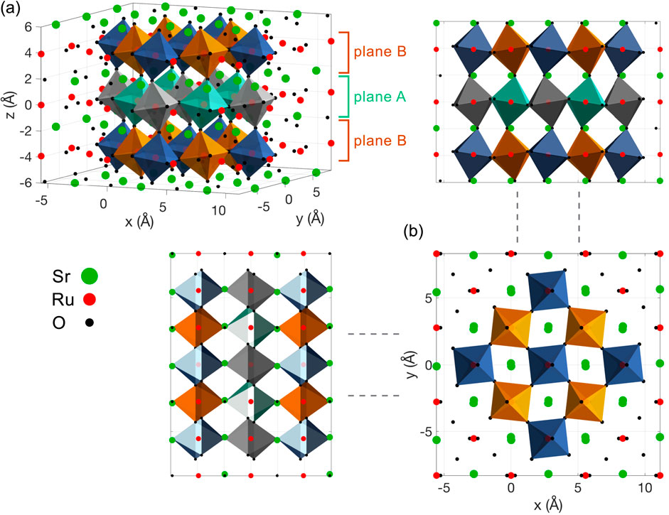
Figure 7. Parametrization of the octahedra in ${\mathrm{S}\mathrm{r}\mathrm{R}\mathrm{u}\mathrm{O}}_3$ using the 4-octahedral model. (A) Visualization of the crystal lattice, where two distinct planes of corner-sharing octahedra have been identified. (B) Different projections of the octahedra in (A), evidencing the symmetry of the octahedral configuration.

The reader is encouraged to test this by running SrRuO3_lattice.m in the MATLAB command window. The first part of the routine builds the ${\mathrm{S}\mathrm{r}\mathrm{R}\mathrm{u}\mathrm{O}}_3$ crystal structure from the available crystallographic information (Gardner et al., 1995), while the second part searches for the octahedral coordinates around the Ru atoms in the selected plane, analyzes them according to the procedure described in Section 1.3, and retrieves the octahedral parameters. A similar example is available for ${\mathrm{N}\mathrm{d}\mathrm{G}\mathrm{a}\mathrm{O}}_3$ (Angel et al., 2007).

2 The 4-Octahedra model under strain

2.1 Constitutive equations

The connection we have established between the global properties of the lattice and the local octahedral configuration allows us to tune the former to derive the possible outcomes of the latter. In experiments involving the epitaxial strain, for example, where an adequate substrate is chosen to vary the in-plane lattice parameters of a specimen layer or heterostructure (Paris et al., 2020), the control is always on the global properties of the lattice, more specifically the lattice vectors. There is no such method (yet) as to manipulate a single octahedron and study its effect on its surroundings. Instead, we tune octahedra indirectly by changing macroscopic parameters. In this context, we can apply the laws of continuum mechanics to the lattice and use the 4-octahedra parametrization to see how these adjustments affect the local octahedral configuration.

Away from strain gradients, such as in the central region of a crystal being compressed by a vice, the strain configuration of a system is characterized by a constant strain tensor. In two dimensions, this corresponds to the knowledge of three quantities $\{{\epsilon }_{xx},{\epsilon }_{yy},{\gamma }_{xy}\}$, which are the longitudinal and shear strains, respectively. To calculate these, it suffices to address the strain configuration of a single 4-octahedron, which repeats itself along the homogeneous region with the same strain values. Therefore, we can build the two-dimensional strain tensor for the parallelogram with corners $\{\mathbf{0},{\mathbf{u}}_1,{\mathbf{u}}_2,{\mathbf{u}}_1+{\mathbf{u}}_2\}$ (see Figure 5). Moreover, while the 4-octahedra is used to generate a two-dimensional lattice, it clearly consists of a three-dimensional object. Motivated by the definition of the tetragonal vectors in Equations 62, 63, we define the vector

$\mathbf{z}=\widehat{k}\bar{\mathbf{P}},(64)$

which represents the extent of the 4-octahedra along the out-of-plane direction, that is, we can think of the vectors $\{{\mathbf{u}}_1,{\mathbf{u}}_2,\mathbf{z}\}$ as the edges of a box delimiting the 4-octahedra. Thus, we build the three-dimensional strain tensor for the parallelepiped formed by the corners of the parallelogram mentioned above and the points $\{\mathbf{z},{\mathbf{u}}_1+\mathbf{z},{\mathbf{u}}_2+\mathbf{z},{\mathbf{u}}_1+{\mathbf{u}}_2+\mathbf{z}\}$. From the finite element method theory, we can write the displacement field $\mathbf{u}=\mathbf{x}-\mathbf{X}$ of a parallelepiped as

$\mathbf{u}=\left(\begin{array}{ccc}\hfill c_{01}\hfill & \hfill c_{02}\hfill & \hfill c_{03}\hfill \end{array}\right)+\mathbf{X}\left(\begin{array}{ccc}\hfill c_{11}\hfill & \hfill c_{12}\hfill & \hfill c_{13}\hfill \\ \hfill c_{21}\hfill & \hfill c_{22}\hfill & \hfill c_{23}\hfill \\ \hfill c_{31}\hfill & \hfill c_{32}\hfill & \hfill c_{33}\hfill \end{array}\right),(65)$

where $(X,Y,Z)$ and $(x,y,z)$ are points of the parallelepiped before and after deformation, respectively, $(u,v,w)$ are the components of $\mathbf{u}$, and the strain fields are given by:

${\epsilon }_{xx}=\frac{\partial u}{\partial X}=c_{11},(66)$

${\epsilon }_{yy}=\frac{\partial v}{\partial Y}=c_{22},(67)$

${\gamma }_{xy}=\frac{1}{2}\left(\frac{\partial u}{\partial Y}+\frac{\partial v}{\partial X}\right)=\frac{c_{21}+c_{12}}{2},(68)$

${\epsilon }_{zz}=\frac{\partial w}{\partial Z}=c_{33},(69)$

${\gamma }_{xz}=\frac{1}{2}\left(\frac{\partial u}{\partial Z}+\frac{\partial w}{\partial X}\right)=\frac{c_{31}+c_{13}}{2},(70)$

${\gamma }_{yz}=\frac{1}{2}\left(\frac{\partial v}{\partial Z}+\frac{\partial w}{\partial Y}\right)=\frac{c_{32}+c_{23}}{2}.(71)$

Evaluating Equation 65 at $\mathbf{X}=\mathbf{0}$ assuming that $\mathbf{u}(\mathbf{0})=\mathbf{0}$ yields $c_{01}=0$, $c_{02}=0$, and $c_{03}=0$.⁵ Using this and Equations 62–64, the equations at the corners $\{{\mathbf{u}}_1,{\mathbf{u}}_2,\mathbf{z}\}$ become, respectively,

$\widehat{i}\left(\bar{\mathbf{P}}-{\bar{\mathbf{P}}}_0\right)=\widehat{i}{\bar{\mathbf{P}}}_0\left(\begin{array}{ccc}\hfill c_{11}\hfill & \hfill c_{12}\hfill & \hfill c_{13}\hfill \\ \hfill c_{21}\hfill & \hfill c_{22}\hfill & \hfill c_{23}\hfill \\ \hfill c_{31}\hfill & \hfill c_{32}\hfill & \hfill c_{33}\hfill \end{array}\right),$

$\widehat{j}\left(\bar{\mathbf{P}}-{\bar{\mathbf{P}}}_0\right)=\widehat{j}{\bar{\mathbf{P}}}_0\left(\begin{array}{ccc}\hfill c_{11}\hfill & \hfill c_{12}\hfill & \hfill c_{13}\hfill \\ \hfill c_{21}\hfill & \hfill c_{22}\hfill & \hfill c_{23}\hfill \\ \hfill c_{31}\hfill & \hfill c_{32}\hfill & \hfill c_{33}\hfill \end{array}\right),$

$\widehat{k}\left(\bar{\mathbf{P}}-{\bar{\mathbf{P}}}_0\right)=\widehat{k}{\bar{\mathbf{P}}}_0\left(\begin{array}{ccc}\hfill c_{11}\hfill & \hfill c_{12}\hfill & \hfill c_{13}\hfill \\ \hfill c_{21}\hfill & \hfill c_{22}\hfill & \hfill c_{23}\hfill \\ \hfill c_{31}\hfill & \hfill c_{32}\hfill & \hfill c_{33}\hfill \end{array}\right),$

where $\bar{\mathbf{P}}$ and ${\bar{\mathbf{P}}}_0$ are the $\bar{\mathbf{P}}$-matrices after and before deformation, respectively⁶. At the remaining corners of the parallelepiped, we obtain equations which are sums of the last identities, and therefore, those are linearly-dependent. Thus, imposing $\bar{\mathbf{P}}$ to be lower triangular⁷ and substituting Equations 66–71 into the last expressions yield

$\mathit{\epsilon }={\bar{\mathbf{P}}}_0^{-1}\bar{\mathbf{P}}-\mathbb{I}=\left(\begin{array}{ccc}\hfill {\epsilon }_{xx}\hfill & \hfill 0\hfill & \hfill 0\hfill \\ \hfill 2{\gamma }_{xy}\hfill & \hfill {\epsilon }_{yy}\hfill & \hfill 0\hfill \\ \hfill 2{\gamma }_{xz}\hfill & \hfill 2{\gamma }_{yz}\hfill & \hfill {\epsilon }_{zz}\hfill \end{array}\right),(72)$

which shows an elegant relationship between the global strain $\mathit{\epsilon }$ and the local octahedral configuration encoded in the $\bar{\mathbf{P}}$-matrices⁸. Moreover, motivated by this result, we define the following matrices:

${\mathit{\epsilon }}^l={\mathbf{L}}_0^{-1}\mathbf{L}-\mathbb{I},(73)$

${\mathit{\epsilon }}^g={\mathbf{G}}_0^{-1}\mathbf{G}-\mathbb{I},(74)$

${\mathit{\epsilon }}^r={\mathbf{R}}_0^{-1}\mathbf{R}-\mathbb{I}.(75)$

Thus, expanding $\bar{\mathbf{P}}$ in Equation 61 in terms of the expressions above, we obtain

$\begin{array}{ll}\hfill \bar{\mathbf{P}}& ={\displaystyle \sum _{A,B}}{\mathbf{L}}_i{\mathbf{G}}_i{\mathbf{R}}_i={\displaystyle \sum _{A,B}}\left({\mathbf{L}}_i^0{\mathbf{G}}_i^0{\mathbf{R}}_i^0\right.+{\mathbf{L}}_i^0{\mathit{\epsilon }}_i^l{\mathbf{G}}_i^0{\mathbf{R}}_i^0+{\mathbf{L}}_i^0{\mathbf{G}}_i^0{\mathit{\epsilon }}_i^g{\mathbf{R}}_i^0+{\mathbf{L}}_i^0{\mathbf{G}}_i^0{\mathbf{R}}_i^0{\mathit{\epsilon }}_i^r\hfill \\ \hfill & +{\mathbf{L}}_i^0{\mathit{\epsilon }}_i^l{\mathbf{G}}_i^0{\mathit{\epsilon }}_i^g{\mathbf{R}}_i^0+{\mathbf{L}}_i^0{\mathit{\epsilon }}_i^l{\mathbf{G}}_i^0{\mathbf{R}}_i^0{\mathit{\epsilon }}_i^r+{\mathbf{L}}_i^0{\mathbf{G}}_i^0{\mathit{\epsilon }}_i^g{\mathbf{R}}_i^0{\mathit{\epsilon }}_i^r+\left.{\mathbf{L}}_i^0{\mathit{\epsilon }}_i^l{\mathbf{G}}_i^0{\mathit{\epsilon }}_i^g{\mathbf{R}}_i^0{\mathit{\epsilon }}_i^r\right),\hfill \end{array}(76)$

and substituting into Equation 72 yields

$\mathit{\epsilon }={\mathit{\epsilon }}^L+{\mathit{\epsilon }}^G+{\mathit{\epsilon }}^R+{\mathit{\epsilon }}^{LG}+{\mathit{\epsilon }}^{LR}+{\mathit{\epsilon }}^{GR}+{\mathit{\epsilon }}^{\mathit{LGR}},(77)$

where

${\mathit{\epsilon }}^L={\bar{\mathbf{P}}}_0^{-1}{\displaystyle \sum _{A,B}}{\mathbf{L}}_i^0{\mathit{\epsilon }}_i^l{\mathbf{G}}_i^0{\mathbf{R}}_i^0,(78)$

${\mathit{\epsilon }}^G={\bar{\mathbf{P}}}_0^{-1}{\displaystyle \sum _{A,B}}{\mathbf{L}}_i^0{\mathbf{G}}_i^0{\mathit{\epsilon }}_i^g{\mathbf{R}}_i^0,(79)$

${\mathit{\epsilon }}^R={\bar{\mathbf{P}}}_0^{-1}{\displaystyle \sum _{A,B}}{\mathbf{L}}_i^0{\mathbf{G}}_i^0{\mathbf{R}}_i^0{\mathit{\epsilon }}_i^r,(80)$

${\mathit{\epsilon }}^{LG}={\bar{\mathbf{P}}}_0^{-1}{\displaystyle \sum _{A,B}}{\mathbf{L}}_i^0{\mathit{\epsilon }}_i^l{\mathbf{G}}_i^0{\mathit{\epsilon }}_i^g{\mathbf{R}}_i^0,(81)$

${\mathit{\epsilon }}^{LR}={\bar{\mathbf{P}}}_0^{-1}{\displaystyle \sum _{A,B}}{\mathbf{L}}_i^0{\mathit{\epsilon }}_i^l{\mathbf{G}}_i^0{\mathbf{R}}_i^0{\mathit{\epsilon }}_i^r,(82)$

${\mathit{\epsilon }}^{GR}={\bar{\mathbf{P}}}_0^{-1}{\displaystyle \sum _{A,B}}{\mathbf{L}}_i^0{\mathbf{G}}_i^0{\mathit{\epsilon }}_i^g{\mathbf{R}}_i^0{\mathit{\epsilon }}_i^r,(83)$

${\mathit{\epsilon }}^{\mathit{LGR}}={\bar{\mathbf{P}}}_0^{-1}{\displaystyle \sum _{A,B}}{\mathbf{L}}_i^0{\mathit{\epsilon }}_i^l{\mathbf{G}}_i^0{\mathit{\epsilon }}_i^g{\mathbf{R}}_i^0{\mathit{\epsilon }}_i^r.(84)$

The decomposition in Equation 77 states that the global strain configuration of the lattice $\mathit{\epsilon }$ can be subdivided into local strains generated from octahedral bond-length changes $({\mathit{\epsilon }}^L)$, octahedral angular distortions $({\mathit{\epsilon }}^G)$, octahedral rigid rotations $({\mathit{\epsilon }}^R)$, and their couplings into mixed strains $({\mathit{\epsilon }}^{LG},{\mathit{\epsilon }}^{LR},{\mathit{\epsilon }}^{GR},{\mathit{\epsilon }}^{\mathit{LGR}})$. Equations 78–84 depend only on the original octahedral configuration (which is usually known) and on the local changes made to the octahedra, encoded in the $\mathbf{L}$, $\mathbf{G}$, and $\mathbf{R}$ matrices in Equations 73–75. Therefore, we have provided a framework to track the possible local outcomes of a global strain configuration; that is, one can distribute the applied strain into different microscopic mechanisms to see how these affect geometry-dependent quantities such as the electronic structure.

2.2 Final 4-octahedral configuration: limit cases

The ultimate goal of this work is to determine the final configuration of the 4-octahedra for a given applied strain. In principle, this is quite straightforward because we can calculate the $\bar{\mathbf{P}}$-matrix of the deformed system using Equation 72:

$\bar{\mathbf{P}}={\bar{\mathbf{P}}}_0\left(\mathbb{I}+\mathit{\epsilon }\right),(85)$

assuming that we know the original geometry of the system $({\bar{\mathbf{P}}}_0)$ and the configuration of the applied strain $(\mathit{\epsilon })$, as it is usually the case in experiments involving strain cells or epitaxial strain. Moreover, because the main theorem of the 4-octahedra stated in Section 1.7 requires calculating the geometric scalar fields $C_1$ and $C_2$, which depend exclusively on the $\bar{\mathbf{P}}$-matrix (see Equations 52, 53), Equation 85 automatically reveals the type of lattice developed by the deformed system.

Nevertheless, the $\bar{\mathbf{P}}$-matrix defined in Equation 61 is not an injective map, in the sense that different $\{\mathbf{L},\mathbf{G},\mathbf{R}\}$ matrices can lead to the same $\bar{\mathbf{P}}$-matrix. To see this more clearly, in the example of the surface of ${\mathrm{S}\mathrm{r}}_2$RuO₄, the same strain configuration can be accommodated through bond-length changes alone, octahedral rotations alone, or a mix of both (Morales et al., 2023). Thus, from here, we proceed in two ways: (1) we perform elastic energy minimization of the possible configurations yielding the same $\bar{\mathbf{P}}$-matrix to determine their likelihood of formation. (2) We define limiting cases of Equation 77, leveraging the fact that the strain can be separated into different microscopic components. The spirit of the first approach has been addressed in the work by Qian et al. (2020). However, this requires assumptions about the strength of the different microscopic mechanisms absorbing the strain, including the knowledge of the elastic potential energy required to distort an oxygen junction. Here, we opt for the second method, where rather than estimating the exact relaxed geometry, we compare the cases where all the strain is absorbed by a particular microscopic channel. Thus, we define the longitudinal limit when $\{{\mathbf{\epsilon }}^l\ne 0,{\mathbf{\epsilon }}^g=0,{\mathbf{\epsilon }}^r=0\}$, the distortional limit when $\{{\mathbf{\epsilon }}^l=0,{\mathbf{\epsilon }}^g\ne 0,{\mathbf{\epsilon }}^r=0\}$, and the rotational limit when $\{{\mathbf{\epsilon }}^l=0,{\mathbf{\epsilon }}^g=0,{\mathbf{\epsilon }}^r\ne 0\}$. From Equation 77 and Equations 78–84, this implies that $\mathit{\epsilon }={\mathit{\epsilon }}^L$, $\mathit{\epsilon }={\mathit{\epsilon }}^G$, and $\mathit{\epsilon }={\mathit{\epsilon }}^R$, respectively. The longitudinal limit addresses the case where all the strain is accommodated by octahedral arm length changes, the distortional limit when it is absorbed solely by octahedral angular distortions, and the rotational limit when it only induces rigid octahedral rotations.

2.3 Final 4-octahedra configuration: longitudinal limit

If $\{{\mathbf{\epsilon }}^l\ne 0,{\mathbf{\epsilon }}^g=0,{\mathbf{\epsilon }}^r=0\}$, from Equations 73–75, $\mathbf{G}={\mathbf{G}}_0$ and $\mathbf{R}={\mathbf{R}}_0$. Therefore, from Equation 76, we have

$\bar{\mathbf{P}}={\mathbf{L}}_A{\mathbf{G}}_A^0{\mathbf{R}}_A^0+{\mathbf{L}}_B{\mathbf{G}}_B^0{\mathbf{R}}_B^0.(86)$

In order to solve for $\{{\mathbf{L}}_A,{\mathbf{L}}_B\}$, we must state the symmetry relationship between the arm lengths at sites A and B. We do this by introducing the diagonal matrix ${\mathbf{S}}^L$, with the property ${\mathbf{L}}_B={\mathbf{L}}_A{\mathbf{S}}^L$:

${\mathbf{L}}_A=\bar{\mathbf{P}}{\left({\mathbf{G}}_A^0{\mathbf{R}}_A^0+{\mathbf{S}}^L{\mathbf{G}}_B^0{\mathbf{R}}_B^0\right)}^{-1}.$

Because the $\bar{\mathbf{P}}$-matrix is a function of the global applied strain (see Equation 85), the solution to the equation above might not exist; that is, the applied strain might not be compatible with introducing only bond length changes in the octahedra. For example, if we consider an initial system of equivalent, undistorted, unrotated octahedra with arm lengths equal to unity (see Figure 6A), then ${\bar{\mathbf{P}}}_0=2\mathbb{I}$ and ${\mathbf{G}}_A^0={\mathbf{R}}_A^0={\mathbf{G}}_B^0={\mathbf{R}}_B^0=\mathbb{I}$. Therefore, from Equations 72, 86, assuming that ${\mathbf{S}}^L=\mathbb{I}$, we have

$\mathit{\epsilon }={\left(2\mathbb{I}\right)}^{-1}\left(2{\mathbf{L}}_A\right)-\mathbb{I}={\mathbf{L}}_A-\mathbb{I},(87)$

which must be diagonal by definition of the $\mathbf{L}$-matrices, meaning that this solution is not compatible with any shear strain (the non-diagonal terms in $\mathit{\epsilon }$). To see if a solution exists, it is useful to treat the elements of $\mathit{\epsilon }$ as scalar fields of the particular geometric parameters being varied. For example, in the longitudinal limit, $\mathit{\epsilon }=\mathit{\epsilon }({\mathbf{L}}_A)=\mathit{\epsilon }(a_A^{\prime },b_A^{\prime },c_A^{\prime })$. The experimental value of $\mathit{\epsilon }$ defines six isosurfaces computed from Equation 72, and a solution exists only if all these isosurfaces intersect, which can be verified numerically. In the example above, the isosurfaces are given by the components of Equation 87

$\left(\begin{array}{ccc}\hfill {\epsilon }_{xx}\hfill & \hfill 0\hfill & \hfill 0\hfill \\ \hfill 2{\gamma }_{xy}\hfill & \hfill {\epsilon }_{yy}\hfill & \hfill 0\hfill \\ \hfill 2{\gamma }_{xz}\hfill & \hfill 2{\gamma }_{yz}\hfill & \hfill {\epsilon }_{zz}\hfill \end{array}\right)=\left(\begin{array}{ccc}\hfill a_A^{\prime }-1\hfill & \hfill 0\hfill & \hfill 0\hfill \\ \hfill 0\hfill & \hfill b_A^{\prime }-1\hfill & \hfill 0\hfill \\ \hfill 0\hfill & \hfill 0\hfill & \hfill c_A^{\prime }-1\hfill \end{array}\right),(88)$

and represented visually in Figure 8. In general, the scalar fields in the longitudinal limit are obtained from Equations 72 and 86 as follows:

$\mathit{\epsilon }={\bar{\mathbf{P}}}_0^{-1}{\mathbf{L}}_A\left({\mathbf{G}}_A^0{\mathbf{R}}_A^0+{\mathbf{S}}_L{\mathbf{G}}_B^0{\mathbf{R}}_B^0\right)-\mathbb{I}.$

Figure 8

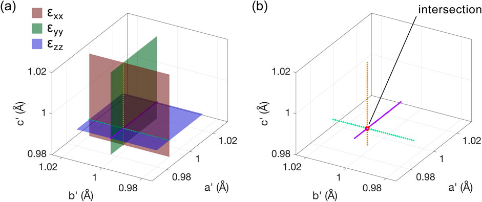
Figure 8. Example solution in the longitudinal limit for a system of equivalent, undistorted, unrotated octahedra with arm lengths equal to unity, subjected to the strain configuration given by $\{{\epsilon }_{xx}=-0.9\%,{\epsilon }_{yy}=0.3\%,{\epsilon }_{zz}=-1.2\%\}$ with no shear. (A) The isosurfaces of the longitudinal strain fields are planes in the space of arm lengths of the A-site. (B) The intersection of the planes yields a unique solution for the arm lengths of the octahedra after deformation. Explicitly, $\{a^{\prime }=0.991,b^{\prime }=1.003,c^{\prime }=0.988\}$, in agreement with Equation 88.

The MATLAB function called Octahedron_strain.m is designed to reproduce this (see Example 1 in the function header) and the following examples in an attempt to provide solutions for the octahedral configuration within the strain limits being discussed.

2.4 Final 4-octahedra configuration: distortional limit

If $\{{\mathbf{\epsilon }}^l=0,{\mathbf{\epsilon }}^g\ne 0,{\mathbf{\epsilon }}^r=0\}$, then $\mathbf{L}={\mathbf{L}}_0$ and $\mathbf{R}={\mathbf{R}}_0$, and the $\bar{\mathbf{P}}$-matrix is given by

$\bar{\mathbf{P}}={\mathbf{L}}_A^0{\mathbf{G}}_A{\mathbf{R}}_A^0+{\mathbf{L}}_B^0{\mathbf{G}}_B{\mathbf{R}}_B^0,$

which we want to solve for $\{{\mathbf{G}}_A,{\mathbf{G}}_B\}$. Thus, introducing the lower-triangular matrix ${\mathbf{S}}^G$, with the property ${\mathbf{G}}_B={\mathbf{G}}_A{\mathbf{S}}^G$, the scalar fields are given by

$\mathit{\epsilon }={\bar{\mathbf{P}}}_0^{-1}\left({\mathbf{L}}_A^0{\mathbf{G}}_A{\mathbf{R}}_A^0+{\mathbf{L}}_B^0{\mathbf{G}}_A{\mathbf{S}}_G{\mathbf{R}}_B^0\right)-\mathbb{I},$

such that $\mathit{\epsilon }=\mathit{\epsilon }({\mathbf{G}}_A)=\mathit{\epsilon }({\alpha }_A^{\prime },{\beta }_A^{\prime },{\gamma }_A^{\prime })$. It can be shown that in the distortional limit, $P_{\mathrm{0,11}}=P_{11}$, and because both ${\bar{\mathbf{P}}}_0$ and $\bar{\mathbf{P}}$ are lower triangular, this implies that ${\epsilon }_{xx}=0$. That is, distortional strain alone cannot induce changes in the $x$-direction, independent of the original configuration of the system. This is a consequence of the particular choice made when fixing the rotational freedom. In general, the $\bar{\mathbf{P}}$-matrix encoding the final configuration does not need to be lower triangular, but it makes sense that at least Equations 58, 59 hold, to guarantee that the applied strain keeps the 4-octahedra within the $xy$-plane.

An example of the distortional limit is given in Figure 9. The starting configuration is the one in Figure 6C, with an in-plane bipartite rotation of 15°. We are interested in a solution with ${\epsilon }_{yy}=-14\%$, ${\epsilon }_{zz}=-7\%$, and no shear strain (see Example 2 in the header of Octahedron_strain.m. Moreover, we impose a symmetry between the A and B sites such that ${\mathbf{G}}_A$ and ${\mathbf{G}}_B$ are related via $\mathrm{\Delta }{\alpha }_A^{\prime }=-\mathrm{\Delta }{\alpha }_B^{\prime }$, $\mathrm{\Delta }{\beta }_A^{\prime }=-\mathrm{\Delta }{\beta }_B^{\prime }$, and $\mathrm{\Delta }{\gamma }_A^{\prime }=-\mathrm{\Delta }{\gamma }_B^{\prime }$, which are the angular deviations from 90° in the respective $\mathbf{G}$-matrices (see Figure 6F for an example of this particular symmetry). In Figures 9A, B, the longitudinal and shear fields have been shown, respectively. Both ${\epsilon }_{xx}$ and ${\gamma }_{xy}$ are not visible: the former is 0 everywhere (as explained before), while the latter vanishes given the symmetry conditions. In Figure 9C, we plot the fields all together, showing that it is impossible to find a solution with both ${\gamma }_{xz}=0$ and ${\gamma }_{yz}=0$. However, we can still find an intersection where the target longitudinal strain values are achieved and only one component of shear strain is non-zero. We choose the solution with ${\gamma }_{yz}=0$, where approximately $\mathrm{\Delta }{\alpha }_A^{\prime }=-20°$, $\mathrm{\Delta }{\beta }_A^{\prime }=$0°, and $\mathrm{\Delta }{\gamma }_A^{\prime }=$19° and plot it in Figure 9D. The reader can verify that the solution has the required strain, except for ${\gamma }_{xz}$ of approximately $9\%$, clearly visible in the output three-dimensional representation of Example 2. In order to incorporate non-zero ${\epsilon }_{xx}$ strain, one must include either octahedral arm length changes or rotations, exhibiting the limited applicability of the distortional limit.

Figure 9

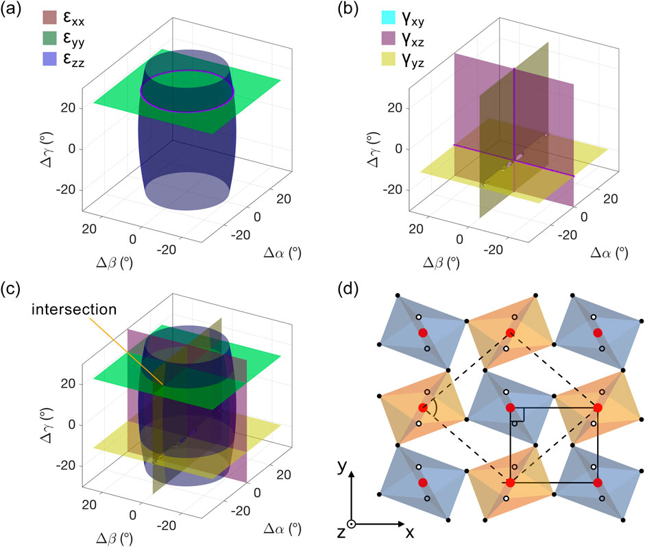
Figure 9. Example solution in the distortional limit for the system of octahedra with in-plane bipartite rotation shown in Figure 6C. (A) Longitudinal strain field isosurfaces for ${\epsilon }_{yy}=-14\%$ and ${\epsilon }_{zz}=-7\%$. (B) Zero shear strain field isosurfaces. (C) All the strain fields combined, showing that only a partial solution can be achieved and requiring at least one non-vanishing component of shear strain. (D) Real space configuration obtained from the intersection in (C), displaying the symmetry imposed over the $\mathbf{G}$-matrices.

2.5 Final 4-octahedra configuration: rotational limit

Finally, if $\{{\mathbf{\epsilon }}^l=0,{\mathbf{\epsilon }}^g=0,{\mathbf{\epsilon }}^r\ne 0\}$, we have $\mathbf{L}={\mathbf{L}}_0$ and $\mathbf{G}={\mathbf{G}}_0$, and the $\bar{\mathbf{P}}$-matrix is given by

$\bar{\mathbf{P}}={\mathbf{L}}_A^0{\mathbf{G}}_A^0{\mathbf{R}}_A+{\mathbf{L}}_B^0{\mathbf{G}}_B^0{\mathbf{R}}_B.$

Because $\bar{\mathbf{P}}$ is lower triangular, we do not need to address the relationship between ${\mathbf{R}}_A$ and ${\mathbf{R}}_B$. It will be given automatically when addressing the rotational freedom. To observe this, from Equations 15, 61, we write $\bar{\mathbf{P}}$ as

$\bar{\mathbf{P}}=\left({\mathbf{L}}_A^0{\mathbf{G}}_A^0{\mathbf{R}}_A^{\prime }+{\mathbf{L}}_B^0{\mathbf{G}}_B^0{\mathbf{R}}_B^{\prime }\right){\mathbf{R}}_f,$

where the matrix in parenthesis is simply ${\bar{\mathbf{P}}}^{\prime }$, the $\bar{\mathbf{P}}$-matrix before the triangularization (see Equation 15). Therefore, we can choose ${\mathbf{R}}_B^{\prime }=\mathbb{I}$, which yields ${\mathbf{R}}_B={\mathbf{R}}_B^{\prime }{\mathbf{R}}_f={\mathbf{R}}_f$ and ${\mathbf{R}}_A={\mathbf{R}}_A^{\prime }{\mathbf{R}}_f={\mathbf{R}}_A^{\prime }{\mathbf{R}}_B$. That is, varying the rotational configuration of one site and addressing the rotational freedom of the system automatically fix the rotational configuration of the other site. Then, in the rotational limit, $\mathit{\epsilon }=\mathit{\epsilon }({\mathbf{R}}_A)=\mathit{\epsilon }({\theta }_A,{\varphi }_A^x,{\varphi }_A^y)$ without any further assumptions, and the scalar fields are given by

$\mathit{\epsilon }={\bar{\mathbf{P}}}_0^{-1}\left({\mathbf{L}}_A^0{\mathbf{G}}_A^0{\mathbf{R}}_A+{\mathbf{L}}_B^0{\mathbf{G}}_A^0{\mathbf{R}}_f\right)-\mathbb{I}.$

The rotational limit in the surface layer of ${\mathrm{S}\mathrm{r}}_2$RuO₄ is explored in Figure 10 with the objective of addressing an experimental situation, originally published in Morales et al. (2023), with a focus on the geometrical details. The surface of ${\mathrm{S}\mathrm{r}}_2$RuO₄ can be modeled as a ${\mathrm{R}\mathrm{u}\mathrm{O}}_2$ layer that exhibits a reconstruction similar to that shown in Figure 6C but with an in-plane rotation of approximately 7°(rather than 15°), octahedral arm lengths deduced from the lattice parameters of the compound, and with Ru in the cages and O at the corners. If we apply uniaxial compression along the $x$-direction in Figure 6C, the strain response of the material is not obvious, and one possibility is that the strain is accommodated by octahedral rotations alone. We are interested in a solution with ${\epsilon }_{xx}=-0.9\%$, ${\epsilon }_{yy}=0.3\%$, and no shear strain: The value of ${\epsilon }_{xx}$ was applied experimentally, ${\epsilon }_{yy}$ is close to the expected Poisson expansion in the perpendicular direction, and the absence of shear is reasonable considering that no de-lamination or domain formation was observed during the straining process.

Figure 10

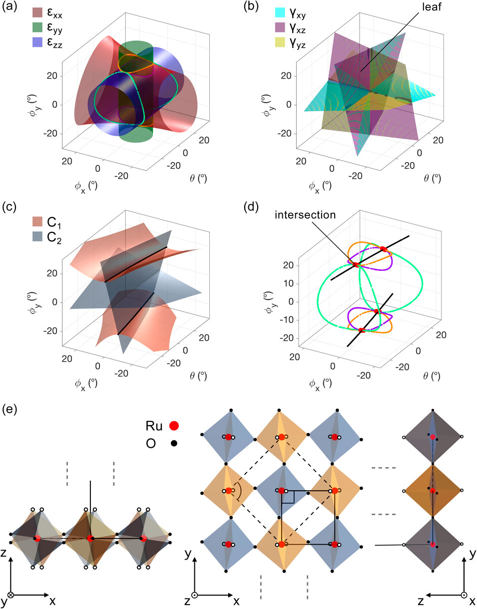
Figure 10. The surface layer of ${\mathrm{S}\mathrm{r}}_2$RuO₄ under uniaxial compression in the rotational limit. (A) Longitudinal strain field isosurfaces for ${\epsilon }_{xx}=-0.9\%$ and ${\epsilon }_{yy}=0.3\%$ and calculated ${\epsilon }_{zz}=-1.2\%$. (B) Zero shear strain field isosurfaces. (C) Geometric field isosurfaces for calculated $C_1=-0.36{\text{Å}}^2$ and $C_2=0{\text{Å}}^2$, leading to a centered orthorhombic configuration. (D) Global isosurface intersection, with ${\gamma }_{yz}=1.4\%$. (E) Calculated strained configuration and its projections along different axes for the solution indicated in (D).

Figures 10A, B show the longitudinal and shear strain field isosurfaces, respectively. The longitudinal isosurfaces intersect in four regions (see the color contours in Figure 10D). The value of ${\epsilon }_{zz}$ is not known experimentally because the development of in-plane rotations results in the shrinkage of the layer along the $z$-direction (so-called auxetic behavior, see the bottom panel in Figure 10E), instead of the typical Poisson expansion. A value of ${\epsilon }_{zz}=-1.2\%$ was required to achieve the intersection of the three longitudinal isosurfaces. Moreover, the shear isosurfaces all intersect only at points away from the intersection of the longitudinal ones. Each leaf in Figure 10B corresponds to the intersection of two shear isosurfaces, yielding the glitch-like texture in the render. A careful analysis of Example 3 in Octahedron_strain.m shows that the leaf where both ${\gamma }_{xy}$ and ${\gamma }_{xz}$ vanish (marked with a line in Figure 10B) contains the intersection of the longitudinal isosurfaces, meaning that a global solution exists as long as ${\gamma }_{yz}\ne 0$. More precisely, ${\gamma }_{yz}=1.4\%$ in this example, which indicates that the rotational limit cannot be reconciled with the absence of layer shearing. The calculated band structure in this limit was shown to be inconsistent with the measured spectroscopy in Morales et al. (2023), and the inevitable development of shear strain might be the reason behind it. Figure 10C shows the geometric field isosurfaces $C_1=-0.36$ and $C_2=0$, calculated from the experimental strain configuration and indicating a centered orthorhombic solution. The $C_1$ isosurface is branched (disjoint), consistent with a non-vanishing value, while $C_2$ forms a joint set in the parameter space. Not surprisingly, their intersection also crosses the global solution (see the black contour in Figure 10D) as $C_1$ and $C_2$ are functions of the strain configuration. Finally, the intersection marked in Figure 10C was used to construct the final octahedral configuration Figure 10E. This shows that the compression in the $x$-direction is alleviated by the introduction of a scissor-like rotation along the $y$-axis, which in turn compresses the layer along the $z$-direction. The ${\gamma }_{yz}$ shear strain in the right-hand side projection is imperceptible in the figure but is clearly present when studied quantitatively in the output visualizations of Example 3. The function Octahedron_strain.m also includes a simple additional Example 4, which deals with the unfolding of in-plane rotation via epitaxial strain in the rotational limit.

2.6 Final 4-octahedra configuration: general case

If a particular system is studied away from the limits above and the global strain is shared between the different microscopic mechanisms described in Equation 77, the procedure to find the solution space becomes quite elaborate. One must build the $\bar{\mathbf{P}}$-matrix of the system and find the intersection of the strain field isosurfaces in each of the three geometric spaces: arm lengths, distortion angles, and rigid rotations, which makes the graphical method quite inefficient. Assuming that the symmetries between the A and B sites are known, up to nine parameters can be varied to achieve a certain strain configuration $(\mathit{\epsilon })$, and their set of values compatible with $\mathit{\epsilon }$ defines the solution. The best approach in this situation is to solve Equation 72 directly, which is a system of six nonlinear equations of the parameters at the A-site. This can be achieved by simplifying the equations analytically and using one of the many numerical methods available in the literature, mostly relying on generalized Newton–Raphson approaches (Remani, 2013). The solution space may be further classified by employing elements of group theory, in a fashion similar to that of references (Howard and Stokes, 1998; Balachandran and Rondinelli, 2013).

3 Discussion

The value of the 4-octahedral model developed in this study can be regarded as technical, experimental, and theoretical. The single octahedron parametrization defined in Sections 1.2 and 1.3 can be readily used to extract the octahedral parameters from many crystal structures and could well be employed to define a standard to measure arm-lengths, orthogonality deviations, rigid rotations, and apical distortions. Furthermore, the general 4-octahedral model built in Sections 1.4–1.8 provides stringent conditions for systems of up to four inequivalent sites to link and form a two-dimensional lattice, while in Section 1.9, we provided a procedure to find such conditions in systems with three dimensions and $N>4$ inequivalent sites. Moreover, a classification of the possible lattice geometries compatible with a particular local octahedral configuration was found in Section 1.7, which can also be extended to three dimensions and $N>4$ inequivalent sites.

The particular case of a bipartite lattice was thoroughly studied and linked to real experimental situations, both for the description of perovskites in Section 1.9 and for the analysis of the surface electronic structure of ${\mathrm{S}\mathrm{r}}_2$RuO₄ under uniaxial compression, explained with great detail in Morales et al. (2023). The latter involved subjecting the bipartite 4-octahedral lattice to general strain, as described in Sections 2.1–2.6. Given the vast extent of the parameter space, final configurations were obtained using a limit approach; however, the general Equations 77, 85 are of significant theoretical value. The former states how lattice strain is decomposed into strains coming from the variation in groups of octahedral parameters in a system described by a $\bar{\mathbf{P}}$-matrix, while the latter describes the evolution of the $\bar{\mathbf{P}}$-matrix itself. That is, these equations hold for any $N$-octahedral system described by a $\bar{\mathbf{P}}$-matrix compatible with the procedure in Section 1.9.

Future work that would considerably enrich this work involves the development of a mathematical framework to efficiently carry out such procedures and methods to find, classify, and study the structure of the large solution space described by Equations 77, 85. On the experimental front, the community already shows signs of interest toward the simulation of low-energy electron diffraction (LEED) patterns, benefiting from the rigorous and systematic control of the octahedral geometry provided in this study.

4 Conclusion

The 4-octahedral model provides a rigorous and tunable parametrization of systems of corner-sharing octahedra. The map between the global properties of the lattice and the local octahedral configuration allows for investigating the microscopic geometric response to applied strain and further classifying it into different mechanisms (see Equation 77). Although two-dimensional in nature, the model can be readily generalized to three dimensions by following a similar approach to the one presented in this study. Furthermore, when used as the geometric input in different types of calculations (ab initio tight binding models (Morales et al., 2023), for example), it provides a powerful and inexpensive benchmark to test the effects that octahedral distortions and rotations have on the electronic structure of many quantum materials.

Data availability statement

The original contributions presented in the study are included in the article/Supplementary Material; further inquiries can be directed to the corresponding author.

Author contributions

EM: writing–original draft and writing–review and editing.

Funding

The author declares that financial support was received for the research, authorship, and/or publication of this article. The author was directly funded by the Max Planck Society as part of their post-doctoral research position at the Max Planck Institute for Chemical Physics of Solids.

Acknowledgments

The author is grateful to Prof. Phil D. C. King for his support and valuable comments during the development of this model and his supervisor Berit H. Goodge for her useful remarks and suggestions during the writing of this manuscript.

Conflict of interest

The author declares that the research was conducted in the absence of any commercial or financial relationships that could be construed as a potential conflict of interest.

Publisher’s note

All claims expressed in this article are solely those of the authors and do not necessarily represent those of their affiliated organizations, or those of the publisher, the editors, and the reviewers. Any product that may be evaluated in this article, or claim that may be made by its manufacturer, is not guaranteed or endorsed by the publisher.

Footnotes

¹The method decomposes a square matrix into a product of an element of $SO(3)$ and an upper triangular matrix.

²Note that $\mathbf{P}$ describes a single octahedron, while $\bar{\mathbf{P}}$ refers to the 4-octahedra.

³Naturally, ${\mathbf{F}}_1={\mathbf{F}}_4={\mathbf{F}}_A$ and ${\mathbf{F}}_2={\mathbf{F}}_3={\mathbf{F}}_B$, but the apical distortions do not play a role in two-dimensional octahedral linking or lattice formation.

⁴These are lattice vectors only if sites A and B are equivalent (see Figure 5).

⁵Without loss of generality, this defines a fixed body point for the displacement field.

⁶In this section, the use of a zero index refers to the original configuration, and its absence refers to the strained system.

⁷That is, we address the global rotational freedom of the strained configuration to match the one of the unstrained system.

⁸Here, $\mathit{\epsilon }$ is not a matrix representation of the strain tensor as it would need to be symmetric, but rather a matrix containing the same information as the strain tensor.

References

Ali, Z., Saghayezhian, M., Wang, Z., O’Hara, A., Shin, D., Ge, W., et al. (2022). Emergent ferromagnetism and insulator-metal transition in delta-doped ultrathin ruthenates. npj Quantum Mater. 7 (1), 108. doi:10.1038/s41535-022-00518-7

CrossRef Full Text | Google Scholar

Angel, R., Zhao, J., Ross, N., Jakeways, C., Redfern, S., and Berkowski, M. (2007). High-pressure structural evolution of a perovskite solid solution (La_1-xNd_x)GaO₃. J. Solid State Chem. 180 (12), 3408–3424. doi:10.1016/j.jssc.2007.09.019

CrossRef Full Text | Google Scholar

Angel, R. J., Zhao, J., and Ross, N. L. (2005). General rules for predicting phase transitions in perovskites due to octahedral tilting. Phys. Rev. Lett. 95 (2), 025503–503. doi:10.1103/physrevlett.95.025503

PubMed Abstract | CrossRef Full Text | Google Scholar

Aso, R., Kan, D., Shimakawa, Y., and Kurata, H. (2013). Atomic level observation of octahedral distortions at the perovskite oxide heterointerface. Sci. Rep. 3 (1), 2214. doi:10.1038/srep02214

PubMed Abstract | CrossRef Full Text | Google Scholar

Balachandran, P. V., and Rondinelli, J. M. (2013). Interplay of octahedral rotations and breathing distortions in charge-ordering perovskite oxides. Phys. Rev. B 88 (5), 054101–101. doi:10.1103/physrevb.88.054101

CrossRef Full Text | Google Scholar

Berner, P. (2008). “Technical concepts: orientation, rotation, velocity and acceleration, and the SRM,” TENA (test & training enabling architecture) project by SEDRIS 21. Tech. Rep.

Google Scholar

Gander, W. (1980). Algorithms for the QR decomposition. Res. Rep. 80 (02), 1251–1268.

Google Scholar

Gardner, J., Balakrishnan, G., and Paul, D. M. (1995). Neutron powder diffraction studies of Sr₂RuO₄ and SrRuO₃. Phys. C. Supercond. 252 (3-4), 303–307. doi:10.1016/0921-4534(95)00495-5

CrossRef Full Text | Google Scholar

Glazer, A. M. (1972). The classification of tilted octahedra in perovskites. Acta Crystallogr. B Struct. Cryst. Cryst. Chem. 28 (11), 3384–3392. doi:10.1107/s0567740872007976

CrossRef Full Text | Google Scholar

Grosso, B. F., and Spaldin, N. A. (2021). Prediction of low-energy phases of BiFeO₃ with large unit cells and complex tilts beyond Glazer notation. Phys. Rev. Mater. 5 (5), 054403–403. doi:10.1103/physrevmaterials.5.054403

CrossRef Full Text | Google Scholar

Hammonds, K. D., Bosenick, A., Dove, M. T., and Heine, V. (1998). Rigid unit modes in crystal structures with octahedrally coordinated atoms. Am. Mineral. 83 (5-6), 476–479. doi:10.2138/am-1998-5-607

CrossRef Full Text | Google Scholar

He, J., Borisevich, A., Kalinin, S. V., Pennycook, S. J., and Pantelides, S. T. (2010). Control of octahedral tilts and magnetic properties of perovskite oxide heterostructures by substrate symmetry. Phys. Rev. Lett. 105 (22), 227203–203. doi:10.1103/physrevlett.105.227203

PubMed Abstract | CrossRef Full Text | Google Scholar

Herklotz, A., Wong, A. T., Meyer, T., Biegalski, M. D., Lee, H. N., and Ward, T. Z. (2016). Controlling octahedral rotations in a perovskite via strain doping. Sci. Rep. 6 (1), 26491–26497. doi:10.1038/srep26491

PubMed Abstract | CrossRef Full Text | Google Scholar

Howard, C. J., and Stokes, H. T. (1998). Group-theoretical analysis of octahedral tilting in perovskites. Acta Cryst. B 54 (6), 782–789. doi:10.1107/s0108768198004200

CrossRef Full Text | Google Scholar

Liao, Z., Huijben, M., Zhong, Z., Gauquelin, N., Macke, S., Green, R. J., et al. (2016). Controlled lateral anisotropy in correlated manganite heterostructures by interface-engineered oxygen octahedral coupling. Nat. Mater. 15 (4), 425–431. doi:10.1038/nmat4579

PubMed Abstract | CrossRef Full Text | Google Scholar

Lu, W., Dong Song, W., He, K., Chai, J., Sun, C. J., Chow, G. M., et al. (2013). The role of octahedral tilting in the structural phase transition and magnetic anisotropy in SrRuO₃ thin film. J. Appl. Phys. 113 (6), 063–901. doi:10.1063/1.4790699

CrossRef Full Text | Google Scholar

Morales, E. A., Siemann, G.-R., Zivanovic, A., Murgatroyd, P. A. E., Marković, I., Edwards, B., et al. (2023). Hierarchy of lifshitz transitions in the surface electronic structure of Sr₂RuO₄ under uniaxial compression. Phys. Rev. Lett. 130 (9), 096–401. doi:10.1103/PhysRevLett.130.096401

CrossRef Full Text | Google Scholar

Paris, E., Tseng, Y., Pärschke, E. M., Zhang, W., Upton, M. H., Efimenko, A., et al. (2020). Strain engineering of the charge and spin-orbital interactions in Sr₂IrO₄. Proc. Natl. Acad. Sci. U.S.A. 117 (40), 24 764–824 770. doi:10.1073/pnas.2012043117

PubMed Abstract | CrossRef Full Text | Google Scholar

Petrov, A. Y., Torrelles, X., Verna, A., Xu, H., Cossaro, A., Pedio, M., et al. (2013). Surface octahedral distortions and atomic design of perovskite interfaces. Adv. Mater. 25 (29), 4043–4048. doi:10.1002/adma.201301841

PubMed Abstract | CrossRef Full Text | Google Scholar

Qian, H., Yu, Z., Lyu, C., Chen, F., Luo, Y., Liu, Y., et al. (2020). Easy-to-use model to reveal the nature of octahedral rotation transformations in perovskites. Ceram. Int. 46 (4), 4477–4483. doi:10.1016/j.ceramint.2019.10.174

CrossRef Full Text | Google Scholar

Remani, C. (2013) Numerical methods for solving systems of nonlinear equations, 77. Ontario, Canada: Lakehead University Thunder Bay.

Google Scholar

Roithmayr, C. M., and Hodges, D. H. (2016). Dynamics: theory and application of kane’s method. J. Comput. Nonlinear Dyn. 11. doi:10.1115/1.4034731

CrossRef Full Text | Google Scholar

Thomas, S., Kuiper, B., Hu, J., Smit, J., Liao, Z., Zhong, Z., et al. (2017). Localized control of Curie temperature in perovskite oxide film by capping-layer-induced octahedral distortion. Phys. Rev. Lett. 119 (17), 177203–203. doi:10.1103/physrevlett.119.177203

PubMed Abstract | CrossRef Full Text | Google Scholar

T. M. Inc. (2022) MATLAB version: 9.13.0 (R2022b). Natick, Massachusetts, United States. Available at: https://www.mathworks.com.

Google Scholar

Woodward, P. M. (1997). Octahedral tilting in perovskites. I. Geometrical considerations. Acta Cryst. B 53 (1), 32–43. doi:10.1107/s0108768196010713

CrossRef Full Text | Google Scholar