Fatigue damage analysis of plain and steel fiber-reinforced concrete material based on a stiffness degradation microplane model

Steel fiber-reinforced concrete material has garnered significant attention in structure design due to its excellent resistance to fatigue damage. The application of the plain concrete microplane model is extended to steel fiber-reinforced concrete by modifying the stress-strain boundary conditions on the microplane and then extended to fatigue damage analysis by considering fatigue-related material stiffness, mainly concerned with tensile damage, mainly concerned with tensile damage. The normal positive strain on the micro-plane is regarded as the fatigue variable, and the fatigue history variable is the accumulation of the fatigue variable during the loading. The relationship between the fatigue history variable and the material stiffness fatigue degradation function is established. In the numerical implementation, the crack band model is combined to reduce the mesh sensitivity caused by strain localization. During the numerical simulation, the parameters of plain concrete, steel fiber-reinforced concrete, and the material fatigue degradation function can be calibrated sequentially, requiring only a few benchmark tests for accurate parameter calibration. The numerical results show that this model can be used for the fatigue damage analysis of plain concrete and steel fiber-reinforced concrete material. It is expected to be used for the refined analysis of concrete structures under complex loading conditions and structural forms in the future, providing convenience to engineering design, evaluation, and optimization.

1 Introduction

Concrete material has a wide range of applications in infrastructure, including bridges, roads, high-rise buildings, and the foundations of power machinery. However, concrete structures are often subjected to cyclic loads, such as traffic (Zhang et al., 2024) and wind, which can lead to material fatigue stiffness degradation (Riyar et al., 2023). This can gradually deteriorate the structural performance, potentially leading to structural failure. Fiber-reinforced concrete material has emerged as a promising solution to improve the durability and safety of concrete structures. Incorporating short fibers, including steel or polypropylene fibers, into fiber-reinforced concrete results in a composite material that exhibits enhanced resistance to cracking, improved toughness, and fatigue properties (Carlesso et al., 2019). It is imperative to investigate the fatigue characteristics of plain and fiber-reinforced concrete and their damage evolution patterns. This is crucial for precisely predicting and assessing the service life of concrete structures and developing adequate maintenance and reinforcement strategies.

As early as the late 19th century, engineers established the S-N curve (Aas-Jakobsen, 1970; Cornelissen, 1984; Miarka et al., 2022) based on experimental data to reflect the fatigue life of concrete at different stress levels. The S-N curve also applies to fiber-reinforced concrete, but it is necessary to consider the fiber type, volume fraction, and orientation effects on fatigue life. The S-N curve is a reasonable method for estimating the anticipated lifespan under disparate stress levels. However, it requires a substantial corpus of experimental data and may not accurately reflect the intricate stress conditions. With the advent of fracture mechanics, the Paris law (Paris and Erdogan, 1963) was introduced to describe the crack propagation rate in plain concrete under constant load. For fiber-reinforced concrete material, the parameters in the Paris law must be adjusted to reflect the hindering effect of fibers on crack propagation. The Paris law is suitable for single crack extension analysis under simple loading conditions, but its application is limited under complex or variable loading. Hillerborg et al. considered a virtual crack in front of a visible crack in concrete and cohesive stress between the interfaces of the virtual crack (Hillerborg et al., 1976). The cohesive zone model simulates the nonlinear fracture behavior of concrete by defining the relationship between the cohesive stress between the crack interfaces and the crack opening displacement and extends the model to fatigue loading by correcting the relationship between the cohesive stress and the crack opening displacement (Gylltoft, 1984). For fiber-reinforced concrete, the cohesive zone model needs to consider further the bridging effect of fibers, which can increase the cohesive stress at the crack surface and thus slow down the crack extension. The damage constitutive model (Marigo, 1985), on the other hand, describes the degradation of the mechanical properties of concrete under repetitive loading from a material microscopic point of view by introducing damage variables, which can be extended to fatigue loading by introducing fatigue history variables and adjusting the damage evolution conditions. This model considers the emergence and expansion of microcracks within concrete and their effect on the overall material properties. For fiber-reinforced concrete, the damage constitutive model needs to consider the effect of fibers on the damage evolution, including the reinforcing and toughening effects of fibers (Li et al., 2024).

In addition to the macro-mechanical modeling of concrete, researchers began to seek breakthroughs in micro-mechanical theories to study concrete constitutive relationships, such as the microplane damage model (Caner and Bažant, 2013a; Caner and Bazant, 2013b). The microplane, which represents a plane perpendicular to any direction at a material point, can describe the interactions between weak planes, cracks, and different defects on microstructures in all directions and can be used to model the inelastic behavior of quasi-brittle materials (e.g., concrete), and has been developed into its seventh version up to the present day. Subsequently, Caner et al. (2013) extended the normal concrete microplane model to fiber concrete by improving the stress-strain boundary conditions on the microplane to describe the pullout and fracture behavior of fibers in fiber-reinforced concrete. Kirane and Bažant (2015) incorporated the fatigue effect into the normal concrete microplane model by introducing a fatigue history variable to quantify the cyclic damage accumulation of the material. However, there is still a lack of microplane models applicable to fatigue damage studies of fiber-reinforced concrete. Although the performance of Engineered Cementitious Composites (ECC) (Lu et al., 2017; Huang et al., 2022; Zhu et al., 2022) and Ultra High-Performance Fiber Reinforced Concrete (UHPFRC) (Wille et al., 2014; Yoo et al., 2017; Nguyen et al., 2023) is higher than that of ordinary fiber-reinforced concrete. However, considering the cost and construction conditions, steel fiber-reinforced concrete specimen (SFRC) (Li et al., 2018; Chu et al., 2023) is still one of the most common FRCs used in engineering. Although compression also leads to fatigue-related material stiffness degradation, this paper will focus on the tensile fatigue damage of SFRC, considering the significant difference between concrete’s tensile and compressive properties.

In the following study, Section 2 presents the basic framework of the microplane damage model for plain concrete, including the three processes of projecting macrostrain to micro-strain, establishing the stress-strain relationship on the microplane, and homogenizing microstress to macro-stress. Section 3 describes how to extend the microplane model from plain concrete to steel fiber-reinforced concrete and how to consider fatigue effects in the microplane damage model. Section 4 summarises the numerical algorithm for the microplane model, parameter calibration, and validation of the concrete microplane damage model. Section 5 compares the fatigue damage analysis of plain and steel fiber-reinforced concrete with experimental results. Section 6 summarises the further research focus. Finally, Section 7 summarises the main conclusions of the paper.

2 Microplane damage model for plain concrete

2.1 A framework for microplane theory

The concrete microplane damage model (Caner and Bažant, 2013a; Caner and Bazant, 2013b) consists of three parts: physical mapping of “macro to micro physical variables,” establishment of constitutive relationship at the micro scale, and homogenization of “micro to macro physical variables,” as shown in Figure 1.

Figure 1

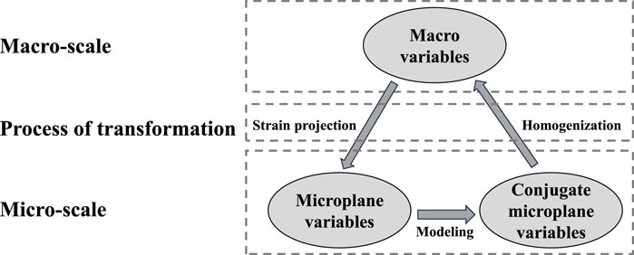
Figure 1. Framework for microplane theory.

2.2 Macroscale to microscale strain decomposition

The microplane model portrays the mechanical behavior of concrete materials at the microscopic level in terms of stresses and strains in vector form, so it is necessary to transform the stresses or strains at the macroscopic level into the stresses or strains at the microscopic level. According to the treatment of the relationship between the macroscopic stress tensor or macroscopic strain tensor and the stress or strain vector on the microplane, they are usually categorized into static and kinematic constraints. They can be understood as the projection of the macroscopic stress tensor on the microplane to obtain the corresponding stress vector and the projection of the macroscopic strain tensor on the microplane to obtain the corresponding strain vector, respectively. Due to the strain-softening behavior of quasi-brittle materials such as concrete, the kinematic constraints shown in Figure 2 are used in the concrete microplane damage model to ensure the stability of the model when analyzing strain softening.

Figure 2

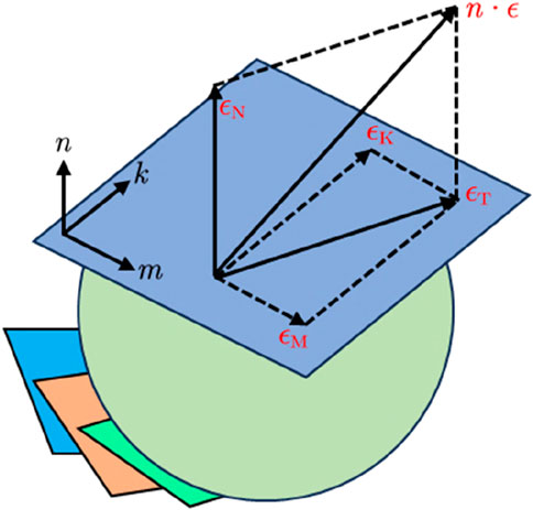
Figure 2. The kinematic constraints.

As shown in Figure 2, the strain vector $\mathit{e}$ on the microplane $i$ (normal vector is denoted as $\mathit{n}$) is expressed as the projection of the macroscopic strain vector $\mathit{ϵ}$ by Equation 1.

$\mathit{e}=\mathit{n}\cdot \mathit{ϵ}=e_N\mathit{n}+e_{\mathrm{T}}(1)$

where $e_N={\mathit{ϵ}}_N=\mathit{N}:\mathit{ϵ}$ is the normal strain component on the microplane, $e_{\mathrm{T}}={\mathit{ϵ}}_{\mathrm{T}}=\mathit{T}\cdot \mathit{ϵ}$ is the tangential shear strain vector on the microplane, $\left|e_{\mathrm{T}}\right|=\sqrt{{\mathit{ϵ}}_K^2+{\mathit{ϵ}}_M^2}$; $\mathit{N}$ and $\mathit{T}$ are the corresponding projection operators. Further, the tangential strain $e_{\mathrm{T}}$ in the microplane is used to characterize plasticity and friction; the normal strain $e_N$ is distinguished into the tensile strain (i.e., the part where $e_N>0$) to characterize the tensile ability, and the compressive strain (i.e., the part where $e_N<0$) to characterize the compressive ability, while the compressive strain can be decomposed into the volume component $e_V$ and the deviatoric component $e_D$ by Equation 2.

$e_N=e_V+e_D=\mathit{V}:\mathit{ϵ}+\mathit{D}:\mathit{ϵ}(2)$

where $\mathit{V}=\frac{1}{3}\mathit{I}$ is the volume component, $\mathit{D}=\mathit{n}\otimes \mathit{n}-\frac{1}{3}\mathit{I}$ denotes the bias obtained by subtracting the volume component from the total strain, and $\mathit{I}$ is the third-order unit tensor.

2.3 Stress-strain relationships on microplane

2.3.1 Elastic response and stiffness degradation

Unlike the traditional tensor-type constitutive model, the microplane model defines constitutive relations on a general plane (microplane) in any direction at a material point. If the strain component on the microplane has been obtained from kinematic constraints, the general expression for the stress on the microplane is given by Equation 3.

$\begin{array}{c}{\sigma }_N\left(t\right)={\mathcal{F}}_{\tau =0}^t\left[{\epsilon }_N\left(\tau \right),{\epsilon }_T\left(\tau \right)\right],\\ {\sigma }_L\left(t\right)={\mathcal{G}}_{\tau =0}^t\left[{\epsilon }_N\left(\tau \right),{\epsilon }_T\left(\tau \right)\right],\\ {\sigma }_M\left(t\right)={\mathcal{H}}_{\tau =0}^t\left[{\epsilon }_N\left(\tau \right),{\epsilon }_T\left(\tau \right)\right].\end{array}(3)$

where $\mathcal{F},\mathcal{G},\mathcal{H}$ is the history functional of the microplane strain at moment $t$.

When the stress on the microplane develops in the elastic range, the normal strain is not decomposed into its volume component $e_V$ and bias component $e_D$, and the modulus of elasticity, shear modulus, and normal strain $e_N$ are used directly to solve for the stress on the microplane. The elasticity modulus $E_N$ and shear modulus $E_T$ on the microplane can be defined as

$E_N=\frac{E}{1-2v},E_T=E_N\frac{1-4\nu }{1+\nu },(4)$

where $E$ is the macroscopic level modulus of elasticity, $\nu$ is Poisson’s ratio, $E_N=K/3$, and $K$ is the bulk modulus. Since $E_N$ and $E_T$ are required to be non-negative, Equation 4 holds for Poisson’s ratio $\nu \in \left[-1,0.25\right]$, and the Poisson’s ratio $\nu$ of concrete (about 0.18) is satisfied. Starting from the microplane model M3 (Bažant et al., 1996), the concept of a stress-strain boundary is introduced, within which the response is considered to be elastic with constant microplane elastic stiffness $E_N$ and $E_T$.

In addition, when the material is in the elastic stage, the modulus of elasticity is gradually degraded due to the progression of damage. The evolution of the microplane normal elastic modulus needs to be considered in the damage variables. Here the current value of the microplane normal elastic modulus damage is calculated by retrieving the largest magnitude of positive and negative normal strains ${ϵ}_N^{0+},{ϵ}_N^{0-}$ stored so far. For the case of ${\sigma }_N^0⩾0$, it is calculated using Equation 5.

$E_N=E_{N0}{e}^{-c_{13}{ϵ}_N^{0+}}f\left(\mathcal{F}\right)\text{\hspace{0.17em}but},E_N=E_{N0},\text{if},{\sigma }_N^0>E_{N0}{ϵ}_N\text{\hspace{0.17em}and\hspace{0.17em}}{\sigma }_N^0∆{ϵ}_N<0(5)$

and in the case of ${\sigma }_N^0<0$, it is calculated using Equation 6.

$E_N=E_{N0}\left(e^{-c_{14}\left|{ϵ}_N^{0-}\right|/\left(1+c_{15}{ϵ}_e\right)}+c_{16}{ϵ}_e\right).(6)$

In Equation 5, the fatigue degradation function $f\left(\mathcal{F}\right)$ and the meaning of the parameters will be described later. At this point the stress in the normal direction of the microplane elastic stage is given by Equation 7.

${\sigma }_N^e={\sigma }_N^0+E_N∆{ϵ}_N,(7)$

It is worth noting that Equation 5 is used in order to ensure that the unloading moves towards the origin along the initial elastic slope after intersection, rather than continuing along the original unloading path after intersection.

2.3.2 Stress-strain boundaries on microplanes

As shown in Figure 2, the strain on the microplane is divided into normal strain and tangential strain, and normal strain can be divided into tensile strain and compressive strain. For normal tensile strain, the tensile normal stress-strain boundary is introduced to characterize the inelastic response on the microplane. For normal compression strain, the key innovation of M7 that significantly improves it is that when the microplane is under pressure, it no longer separately determines whether the volume stress and deviator stress exceed the boundary, but calculates the two boundary values separately and then sums them up, i.e., ${\sigma }_N^b={\sigma }_V^b+{\sigma }_D^b$. Then it is compared with the normal stress ${\sigma }_N^e$ calculated using the elastic increment method to determine the normal stress value on the microplane. The study found this improvement is also logically consistent with elastic and damage potential energy. It effectively avoids problems such as excessive lateral expansion during tensile response and normal stress self-locking in the softening section. In addition, in M7, the boundary function about the shear resultant force ${\sigma }_{\tau }$ is defined, which solves the problem of direction dependence of the results due to the arbitrary selection of shear component coordinates. Therefore, in the microplane model M7 (Caner and Bažant, 2013a; Caner and Bazant, 2013b), the boundary functions that characterize the inelastic response on the microplane are normal tensile stress-strain boundary, compressive deviatoric stress-strain boundary, compressive volume stress-strain boundary and plastic-friction stress-strain boundary (shear boundary).

2.3.2.1 Normal tensile stress-strain boundary

Figure 3A shows that the normal tensile stress-strain boundary controls the tensile fracture behavior, calculated by Equation 8.

${\sigma }_N^b=E{k}_1{\beta }_1{e}^{-〈{ϵ}_N-{\beta }_1{c}_2{k}_1〉/\left(c_4{ϵ}_e\text{sgn}\left({ϵ}_e\right)+k_1{c}_3\right)}.(8)$

where ${\beta }_1=-c_1+c_{17}{e}^{-c_{19}〈{ϵ}_e-c_{18}〉}$. The recommended values of the parameters and their significance in this section will be described in detail later.

Figure 3

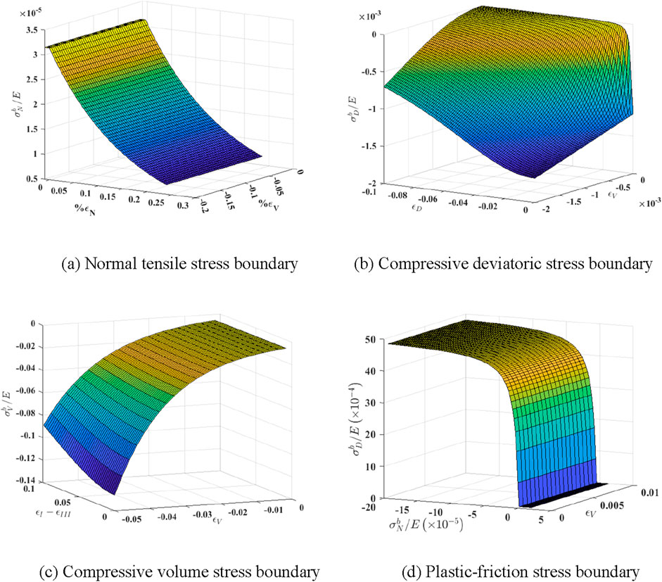
Figure 3. Stress-strain boundaries on the microplane. (A) Normal tensile stress boundary. (B) Compressive deviatoric stress boundary. (C) Compressive volume stress boundary. (D) Plastic-friction stress boundary.

2.3.2.2 Compressive deviatoric stress-strain boundary

Figure 3B shows that the compression deviatoric stress-strain boundary is used to model the damage evolution under compression conditions, calculated by Equation 9.

${\sigma }_D^b=-\frac{E{k}_1{\beta }_3}{1+{\left[〈-{ϵ}_D〉/\left(k_1{\beta }_2\right)\right]}^2}.(9)$

where ${\gamma }_0=f_{c0}^{\prime }/E_0-f_c^{\prime }/E$, ${\gamma }_1=e^{{\gamma }_0}\tanh \left(c_9〈-{ϵ}_V〉/k_1\right)$, ${\beta }_2=c_5{\gamma }_1+c_7$, ${\beta }_3=c_6{\gamma }_1+c_8$. $f_c^{\prime }$ denotes the compressive strength of the concrete material, and $f_{c0}^{\prime }$ is the reference value of compressive strength for model calibration.

2.3.2.3 Compressive volume stress-strain boundary

As shown in Figure 3C, the compressive volumetric stress-strain boundary is used to model pore collapse and expansion rupture of the material, calculated by Equation 10.

${\sigma }_V^b=-E{k}_1{k}_3{e}^{-\frac{{ϵ}_V}{k_1\alpha }},(10)$

where $\alpha =\frac{k_5}{1+{ϵ}_e}{\left(\frac{{ϵ}_I^0-{ϵ}_{III}^0}{k_1}\right)}^{c_{20}}+k_4$. ${ϵ}_I^0,{ϵ}_{III}^0$ are the maximum and minimum principal strains at the beginning of the step, and ${ϵ}_e=〈-{\sigma }_V^0/E_{N0}〉$, where $〈x〉=\max \left(x,0\right)$.

2.3.2.4 Plastic-friction stress-strain boundary (shear boundary)

As shown in Figure 3D, the plastic-friction boundary is used to model the shear behavior of the material, calculated by Equation 11.

${\sigma }_T^b=F_T\left(-{\sigma }_N\right)=\frac{E_T{k}_1{k}_2{c}_{10}〈-{\sigma }_N+{\sigma }_N^0〉}{E_T{k}_1{k}_2+c_{10}〈-{\sigma }_N+{\sigma }_N^0〉}.(11)$

where ${\sigma }_N^0=〈E_T{k}_1{c}_{11}-c_{12}〈{ϵ}_V〉〉$.

2.3.3 Yielding and plastic flow criteria on microplane

The yield condition and plastic flow criterion on the microplane are defined as follows: when the stress on the microplane lies within the stress-strain boundary, the stress-strain on the microplane is in the elastic phase. At this time, the stress is given by ${\sigma }_N^e$ in Equation 7. When the stress on the microplane exceeds the stress-strain boundary, the strain remains, and the stress falls back to the boundary. The normal stress is evaluated using Equation 12.

${\sigma }_N=\max \left[\min \left({\sigma }_N^e,{\sigma }_N^b\right),{\sigma }_V^b+{\sigma }_D^b\right].(12)$

The shear stress on the microplane is given by Equation 13.

${\sigma }_{\tau }=\min \left(\left|{\sigma }_{\tau }^e\right|,{\sigma }_{\tau }^b\right).(13)$

Where the incremental, cumulative form of the formula for calculating the shear stress in the elastic phase on the microplane is given by Equations 14–16.

${\sigma }_{\tau }^e=\sqrt{{\left({\sigma }_M^0+E_T∆{ϵ}_M\right)}^2+{\left({\sigma }_L^0+E_T∆{ϵ}_L\right)}^2},(14)$

${\sigma }_M={\sigma }_M^0+∆{\sigma }_M,{\sigma }_L={\sigma }_L^0+∆{\sigma }_L,(15)$

$∆{\sigma }_M=E_T∆{ϵ}_M\frac{{\sigma }_{\tau }}{{\sigma }_{\tau }^e},∆{\sigma }_L=E_T∆{ϵ}_L\frac{{\sigma }_{\tau }}{{\sigma }_{\tau }^e}.(16)$

2.4 Homogenization from microscale to macroscale

After defining the stress-strain relationship on the microplane, the principle of virtual work is applied to establish the equation between the microplane stress vector and the macroscopic stress tensor, from which the macroscopic stress tensor ${\sigma }_{ij}$ satisfies Equation 17.

$\frac{2\pi }{3}{\sigma }_{ij}\delta {\epsilon }_{ij}={\int }_{\mathrm{\Omega }}\left({\sigma }_N\delta {\epsilon }_N+{\sigma }_L\delta {\epsilon }_L+{\sigma }_M\delta {\epsilon }_M\right)d\mathrm{\Omega }(17)$

where $\mathrm{\Omega }$ is the surface of the unit hemisphere and $2\pi /3$ is the volume of the hemisphere, the integral is regarded as a homogenization of the microplane contributions in different directions within the material. Due to $\delta {\epsilon }_N=N_{ij}\delta {\epsilon }_{ij},\delta {\epsilon }_L=L_{ij}\delta {\epsilon }_{ij}$ and $\delta {\epsilon }_M=M_{ij}\delta {\epsilon }_{ij}$, from the arbitrariness of the variation $\delta {\epsilon }_{ij}$, the equilibrium relation can be obtained as Equations 18, 19.

${\sigma }_{ij}=\frac{3}{2\pi }{\int }_{\mathrm{\Omega }}{s}_{ij}d\mathrm{\Omega }\approx 6{\sum }_{\mu =1}^{N_m}{w}_{\mu }{s}_{ij}^{\left(\mu \right)}(18)$

$s_{ij}={\sigma }_N{N}_{ij}+{\sigma }_L{L}_{ij}+{\sigma }_M{M}_{ij},(19)$

The integral is approximated by the optimal Gaussian integral formula for the sphere, denoting the weighted sum of microplane in the direction ${\mathit{n}}_{\mu }$, with the weight $w_{\mu }$ normalized, so ${\sum }_{\mu }{w}_{\mu }=1/2$. For better accuracy in the far-peak post-softening, 37 microplane are recommended to be preferred.

3 Microplane model extend to steel fiber-reinforced concrete and fatigue damage

3.1 Extend to fiber-reinforced concrete

The simplest way to extend the plain concrete microplane model to make it applicable to SFRC containing materials such as steel fibers is to adjust the stress-strain boundary conditions on the microplane (Caner et al., 2013). First, fibers usually increase the tensile capacity of the concrete material (Jiang et al., 2023; Lakavath et al., 2024), so the effect of steel fiber reinforcement needs to be introduced on the normal tensile stress-strain boundary. The contribution of fiber reinforcement is given by a simplified form of the Kholmyansky equation (Kholmyansky, 2002), as Equation 20.

${\sigma }_N^f=\left\{\begin{array}{l}E{p}_1{k}_1〈{ϵ}_N/k_1〉e^{-p_2〈{ϵ}_N/k_1〉},\text{if\hspace{0.17em}}{ϵ}_N/k_1<1/p_2+p_4.\\ E{p}_1{k}_1/p_2{e}^{-1},\text{if\hspace{0.17em}}1/p_2+p_4⩽{ϵ}_N/k_1<p_3.\\ E{p}_1{k}_1〈{ϵ}_N/k_1-p_3+1/p_2〉e^{-p_2〈{ϵ}_N/k_1-p_3+1/p_2〉},\text{if\hspace{0.17em}}{p}_3⩽{ϵ}_N/k_1.\end{array}\right.(20)$

This contribution is obtained by the gradual activation of the bridging of the fibers during the development of the crack, as shown in Figure 4. Assuming parallel coupling of the fibers and the matrix, the normal stress on the microplane is Equation 21.

${\sigma }_N^{bf}={\sigma }_N^b+{\sigma }_N^f.(21)$

where ${\sigma }_N^{bf}$ is the total normal stress of the fiber-reinforced concrete, ${\sigma }_N^b$ is the normal stress of the plain concrete matrix, and ${\sigma }_N^f$ is the normal stress of steel fiber contribution given by Equation 20. Therefore, in the microplane model of fiber-reinforced concrete, Equation 12 is modified as Equation 22.

${\sigma }_N=\max \left[\min \left({\sigma }_N^e,{\sigma }_N^{bf}\right),{\sigma }_V^b+{\sigma }_D^b\right].(22)$

Figure 4

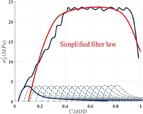
Figure 4. Simplified total fiber law obtained by superimposing multiple fiber responses.

In addition, the tensile capacity that steel fiber-reinforced concrete can withstand changes (increases or decreases) before cracks develop. Therefore, the normal tensile stress-strain boundary Equation 8 of the plain concrete matrix needs to be adjusted to Equation 23.

${\beta }_1=-c_1+c_{17}{e}^{-c_{19}〈{ϵ}_e-c_{18}〉}+p_0\left(V_f\right).(23)$

Secondly, the addition of steel fibers changes the compressive capacity of the concrete material, especially the shear expansion deformation, so the compressive deviatoric stress-strain boundary condition Equation 9 needs to be adjusted to Equation 24.

${\beta }_2=c_5{\gamma }_1+c_7\left(V_f\right).(24)$

Finally, steel fibers change the mechanical behavior of concrete in triaxial compression, so the plastic-friction boundary Equation 11 needs to be adjusted to Equation 25.

${\sigma }_T^b=F_T\left(-{\sigma }_N\right)=\frac{E_T{k}_1{k}_2\left(V_f\right)c_{10}\left(V_f\right)〈-{\sigma }_N+{\sigma }_N^0〉}{E_T{k}_1{k}_2\left(V_f\right)+c_{10}\left(V_f\right)〈-{\sigma }_N+{\sigma }_N^0〉},(25)$

where ${\sigma }_N^0=〈E_T{k}_1{c}_{11}\left(V_f\right)-c_{12}\left(V_f\right)〈{ϵ}_V〉〉〉$.

The microplane model of steel fiber-reinforced concrete is based on the microplane model of plain concrete. Therefore to calibrate its parameters, it is necessary to calibrate the parameters of plain concrete first. Then from the uniaxial tensile data of SFRC, $p_0\left(V_f\right)$, $p_1\left(V_f\right)$, $p_2\left(V_f\right)$, $p_3\left(V_f\right)$, $p_4\left(V_f\right)$ can be identified. From Equation 23, it can be found that the parameter $p_0\left(V_f\right)$ determines whether the fibers in the concrete matrix are bonded or not. The parameter $p_1\left(V_f\right)$ controls the proportion of steel fiber contribution, while $p_2\left(V_f\right)$ controls the pullout of fibers connecting the open cracks. Parameters $p_3\left(V_f\right)$, $p_4\left(V_f\right)$ determine the length of the plastic plateau in the stress-strain relationship (shown in Figure 4). $c_7\left(V_f\right),c_{12}\left(V_f\right)$ can be determined from the uniaxial compression data and $k_2\left(V_f\right),c_{10}\left(V_f\right),c_{11}\left(V_f\right)$ can be determined from triaxial compression data. In many practical applications, fewer triaxial compression problems are involved. Therefore, it is mostly sufficient to study the uniaxial compression and uniaxial tension of fiber concrete. If uniaxial tension tests are difficult to perform, the parameters can be calibrated indirectly by means of the notched three-point loaded bending concrete beam test.

3.2 Extend to fatigue damage

In the concrete microplane damage model, taking the stretch shown in Equation 5 as an example, the damage behavior of concrete under several cycles can be described by assuming that the elastic modulus $E_N$ in the $\mu$-th microplane will undergo damage by Equation 26.

$\frac{E_N\left(\mu \right)}{E_{N0}}=\exp \left(-A{ϵ}_N^{0+}\left(\mu \right)\right).(26)$

where $E_{N0}$ is the undamaged modulus, $A$ is the material parameter which is called $c_{13}$ in Equation 5, and ${ϵ}_N^{0+}\left(\mu \right)$ is the maximum strain reached so far in the $\mu$-th microplane. This approach can characterize the damage to the concrete for a few cycles or so, but it does not capture fatigue. It is worth noting that once damage begins to occur in the material, strain localization occurs, and strain calculations at this point are affected by the finite element mesh size in a way that is difficult to ignore. Therefore, it is necessary to analyze the microplane model in conjunction with nonlocal theory or the crack band model (Bažant and Oh, 1983) (used here). In order to effectively predict the fatigue response, it is necessary to introduce a variable that measures the fatigue damage history paths (Kirane and Bažant, 2015; Baktheer et al., 2021; Aguilar et al., 2022).

3.2.1 Fatigue history variable

The fatigue damage variable is denoted as $\zeta$. $\mathcal{F}$ is the fatigue history variable obtained from the accumulation of fatigue damage variables, and because fatigue damage is irreversible, $\mathcal{F}$ never decreases. For simplicity, in this paper, only the cyclic cumulative damage under tension is considered,and the cyclic cumulative damage under compression is ignored. The normal positive strain ${ϵ}_N^{+}\left(\mu \right)$ reached on the microplane is adopted as the fatigue variable. Then the fatigue damage history variable at the end of the increment is given by Equation 27.

$\mathcal{F}={\mathcal{F}}_0+d\zeta ,d\zeta =\left|d{ϵ}_N^{+}\right|.(27)$

The fatigue damage behavior of concrete under compressive loading can be used as a fatigue variable for compressive fatigue damage by using the normal negative strain, ${ϵ}_N^{-}\left(\mu \right)$, as the fatigue variable for compressive fatigue damage. At this time the elastic model of fatigue damage occurring on the microplane should be calculated using Equation 6.

3.2.2 Fatigue damage estimation

Next, the stiffness degradation of the material is related to the fatigue damage history variables. A model is obtained that is suitable for both fatigue damage analyses without affecting the calibration of the parameters of the original microplane model. The material stiffness degradation on the microplane is represented by the damage parameter $\omega =E_N/E_{N0}$, in for the intact material $\omega =1$, and $\omega =0$ for the fully damaged material. Equation 26 is further written as Equation 28.

$\frac{E_N}{E_{N0}}=\omega =\exp \left(-A{ϵ}_N^{0+}\right).(28)$

Then, introduce $\omega ={\omega }_{\text{cyc}}=f\left(\mathcal{F}\right)$ as the material stiffness degradation due to cyclic loading. To obtain the dependence of the damage parameter $\omega$ on the fatigue history variable $\mathcal{F}$, in analogy with Paris law, the following successively increasing damage accumulation rates are introduced,

$\frac{d{\omega }_{\text{cyc}}}{d\mathcal{F}}=-s{\mathcal{F}}^p.(29)$

where $s$ and $p$ are material parameters. Integration of Equation (29), taking into account $\mathcal{F}=0$ at ${\omega }_{\text{cyc}}=1$, yields

${\omega }_{\text{cyc}}=1-\frac{s}{p+1}{\mathcal{F}}^{p+1}(30)$

Usually taking $p\ge 1$, then Equation (30) becomes negative as the fatigue damage history variable increases. Therefore, the following alternatives are used

${\omega }_{\text{cyc}1}=\frac{1}{1+{\left(s\mathcal{F}\right)}^p+{\left(s\mathcal{F}\right)}^{2p}}(31)$

${\omega }_{\text{cyc}2}=\frac{s{\zeta }_t}{{\mathcal{F}}^p+s{\zeta }_t}(32)$

Similarly, $s$ and $p$ are material parameters that characterize fatigue degradation. ${\zeta }_t$ is the reference strain for uniaxial tensile and ${\zeta }_t=f_t/E_0$ is suggested, where $f_t$ is the material tensile strength. The degradation functions Equations 31, 32 both satisfy the conditions ${\omega }_{\text{cyc}}^{\prime }⩽0$, ${\omega }_{\text{cyc}}⩾0$, and $\underset{\zeta \to \infty }{\lim }{\omega }_{\text{cyc}}=0$. Equations 30–32 correspond to the material fatigue damage softening law as shown in Figure 5. It can be found that the fitting of the test data under monotonic loading is not affected by the degradation function ${\omega }_{\text{cyc}}\approx 1$, due to the small fatigue history variable $\mathcal{F}$, in the first one or two cycles.

Figure 5

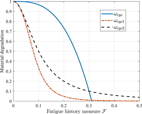
Figure 5. Fatigue degradation law of material $\left(s=100,q=2,{\zeta }_t=0.0001\right)$.

4 Numerical implementation, parameter calibration and model validation

4.1 Numerical implementation

In the numerical implementation, it is necessary to incorporate the crack band model to reduce the mesh size sensitivity of the computed results (Bažant and Oh, 1983; Červenka et al., 2005). In ABAQUS commercial finite element software, VUMAT subroutine is written for numerical implementation. If the stress tried exceeds the stress-strain boundary, it is necessary to keep the strain and limit the stress to the stress-strain boundary. In the finite element method program, if the strain increment $∆{\epsilon }_{ij}$ at the current step is known, as well as the strain ${\epsilon }_{ij}^0$ and stress ${\sigma }_{ij}^0$ at the end of the previous step, the new stress ${\sigma }_{ij}$ is obtained at the end of the current step by the following steps:

Step 1. First, the strain and strain increment on the microplane are calculated by Equation 33 according to Equation 1,

$\mathbf{∆}{\mathbf{\epsilon }}_{\mathbf{N}}\mathbf{=}{\mathbf{N}}_{\mathbf{i}\mathbf{j}}\mathbf{∆}{\mathbf{\epsilon }}_{\mathbf{i}\mathbf{j}}\mathbf{,}∆{\mathbf{\epsilon }}_{\mathbf{M}}\mathbf{=}{\mathbf{M}}_{\mathbf{i}\mathbf{j}}\mathbf{∆}{\mathbf{\epsilon }}_{\mathbf{i}\mathbf{j}},∆{\mathbf{\epsilon }}_{\mathbf{L}}\mathbf{=}{L}_{\mathbf{i}\mathbf{j}}\mathbf{∆}{\mathbf{\epsilon }}_{\mathbf{i}\mathbf{j}}.(33)$

Step 2. Calculate the volumetric strain and its increment at the end of the previous and current steps, based on the given strain and its increment by Equation 34.

${\epsilon }_V^o={\epsilon }_{kk}/3,∆{\epsilon }_V=∆{\epsilon }_{kk}/3,{\epsilon }_V={\epsilon }_V^o+∆{\epsilon }_V.(34)$

Then, calculate ${\epsilon }_e=〈-{\sigma }_V^0/E_{N0}〉$, while the corresponding volumetric stress-strain boundaries ${\sigma }_V^b$ are later calculated by Equation 10. The deviatoric strain can be obtained from total strain and volumetric strain by Equation 35.

$∆{\epsilon }_D=∆{\epsilon }_N-∆{\epsilon }_V,{\epsilon }_D^0={\epsilon }_N-{\epsilon }_V^0,{\epsilon }_D={\epsilon }_D^0+∆{\epsilon }_D,(35)$

and ${\sigma }_D^b$ is calculated by Equation 9.

Step 3. Calculate the ${\epsilon }_N={\epsilon }_V+{\epsilon }_D$ retrieve the history variables ${\epsilon }_N^{0+},{\epsilon }_N^{0-}$ of the largest magnitude stored so far. Next, the current damage degree of the normal elastic modulus of the microplane is calculated according to $E_{N0}=E/\left(1-2\nu \right)$ by Equations 5, 6. Calculating the normal elastic stress of the microplane by Equation 36.

${\sigma }_N^e={\sigma }_N^o+E_N∆{\epsilon }_N(36)$

Step 4. Calculate the normal tensile boundary ${\sigma }_N^b$ of the microplane using Equation 8 when ${\sigma }_N^b>0$.

Step 5. Holding the strain constant and allowing the stress to drop vertically to the normal tensile stress-strain boundary by Equation 37.

${\sigma }_N=\max \left[\min \left({\sigma }_N^e,{\sigma }_N^b\right),{\sigma }_V^b+{\sigma }_D^b\right](37)$

Meanwhile, update the history maxima ${\epsilon }_N^{0+}$ and ${\epsilon }_N^{0+}$.

Step 6. Calculate an approximation of the current volumetric stress by Equation 38.

${\sigma }_V\approx \frac{1}{2\pi }{\displaystyle {\sum }_{\mu =1}^{N_m}}{w}_{\mu }{\sigma }_N(38)$

Retrieve the originally stored microplane shear stresses ${\sigma }_L^o$, ${\sigma }_M^o$, followed by estimating $E_T$ according to Equation 4, and ${\widehat{\sigma }}_N^0=E_T〈k_1{c}_{11}-c_{12}〈{\epsilon }_V〉〉$. If we want to simulate cell failure, the recommended deletion criterion of the adopted cell is ${\epsilon }_I\ge 0.5\%$. The shear boundary is then calculated by Equation 11.

Step 7. Calculate the shear response upon return to the stress-strain boundary by Equations 12–16.

Step 8. The stress ${\sigma }_{ij}$ at the end of the current step is obtained by calculating the sum of stresses on all microplanes through Equations 18, 19, while recording the variables ${\sigma }_V$, ${\sigma }_N$, ${\sigma }_L$, ${\sigma }_M$, ${\epsilon }_N^{0+}$, ${\epsilon }_N^{0-}$ at the end of the current step.

4.2 Parameter calibration

In the microplane model (M7), the shape of the response curve is determined by five free parameters and twenty-one fixed parameters. Tables 1, 2 provide a concise explanation of the meaning and default value of each parameter. The fixed parameters, as detailed in Table 1, are calibrated using the uniaxial compressive strength $f_c^{\prime }=36\text{MPa}$ and the axial normal strain ${\epsilon }_p=0.0036$ at peak stress. The calibration of the uniaxial compressive strength $f_c^{*}$, and the corresponding strain ${\epsilon }_p^{*}$, of a particular concrete using a microplane model requires only that the reference values of the free parameter $k_1$, and the elastic modulus $E$, be modified to,

$k_1^{*}=k_1\frac{{\epsilon }_p^{*}}{{\epsilon }_p},E^{*}=E\frac{f_c^{*}}{f_c^{\prime }}\frac{{\epsilon }_p}{{\epsilon }_p^{*}}.(39)$

Table 1

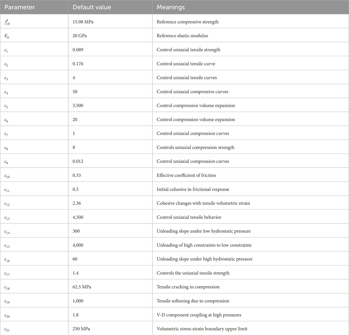
Table 1. Default values of fixed parameters of microplane model and their meaning.

Table 2

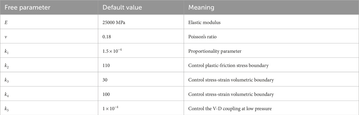
Table 2. Default values of free parameters of microplane model and their meaning.

To optimize the fitting of a large amount of experimental data, it is not necessary to change all five free parameters simultaneously in the actual microplane model (Caner and Bažant, 2013a; Caner and Bazant, 2013b). The elastic modulus $E$ and Poisson’s ratio $v$ are determined through experimental measurement. First, all other parameters are assumed to be reference values, and subsequent parameter calibration is conducted. The parameter $k_1$ was calibrated based on the strain corresponding to the peak stress in the uniaxial compression experiment. If sufficient triaxial compression data are available, and the compression intensity is sufficiently strong to elicit an almost plastic response, the data are fitted by adjusting $k_2$. The parameters $k_3$ and $k_4$ are calibrated based on hydrostatic pressure experimental data. If sufficient uniaxial, biaxial, and triaxial compression data at low hydrostatic pressure are available, $k_5$ should be determined by fitting. Otherwise, the default values are retained.

4.3 Validation of representative examples

4.3.1 Plain concrete specimen

First, the uniaxial compression test of Chern et al. (1993) was fitted to the elastic modulus $E=20\text{GPa}$, compressive strength $f_c^{\prime }=20.65\text{MPa}$, and Poisson’s ratio $\nu =0.18$ of plain concrete materials. The strain ${\epsilon }_p^{*}=0.001458$ corresponding to the peak load was obtained from the uniaxial compression experiment, and the free parameters $k_1=60$ were adjusted according to the prediction Equation 39 proposed by Bazant et al., with other parameters kept defaults. The calculated uniaxial compression stress-strain curve of plain concrete is shown in Figure 6, which is similar to the experimental results.

Figure 6

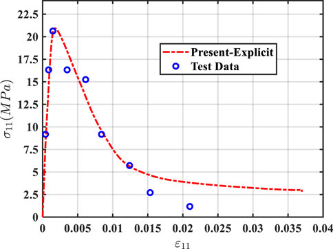
Figure 6. Uniaxial compressive stress-strain curve of plain concrete.

Next, a triaxial compression experiment of concrete under hydrostatic pressure was fitted. Plain concrete material parameters (Chern et al., 1993): elastic modulus $E=20\text{GPa}$, Poisson’s ratio $\nu =0.18$. The free parameter $k_1=60\times 10^{-6}$ and other parameters are kept as default. The simulation and experimental results are shown in Figure 7A. The model is sufficient to capture concrete compression under low hydrostatic pressure conditions. Therefore, it is suitable for capturing the nonlinear behavior of concrete under conventional conditions.

Figure 7

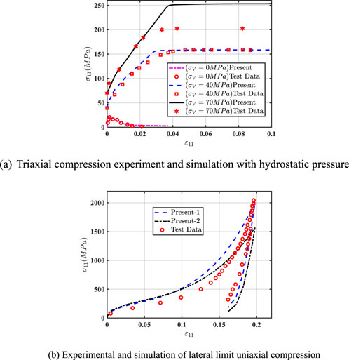
Figure 7. Experimental and simulation of compression. (A) Triaxial compression experiment and simulation with hydrostatic pressure. (B) Experimental and simulation of lateral limit uniaxial compression.

Then, the mechanical behavior of plain concrete under side-limited uniaxial compression was fitted. The plain concrete material parameters (Caner and Bazant, 2013a): elastic modulus $E=41.369\text{GPa}$, Poisson’s ratio $\nu =0.18$, free parameters $k_1=105\times 10^{-6}$, $k_3=10$, $k_4=150$, and other parameters are kept default. The simulation results are shown in Present-1 in Figure 7B, which agrees with the tests. In literature (Caner and Bazant, 2013b), the free parameter $k_1=120\times 10^{-6}$, corresponding to the computational results as shown in Present-2 in Figure 7B. When microplane model parameters are calibrated, it can be well used to capture plain concrete mechanical response.

4.3.2 Steel fiber-reinforced concrete specimen

In this section, the mechanical response of steel fiber-reinforced concrete is analyzed. The parameter calibration was performed for fiber reinforced, as shown in Table 3 (Caner et al., 2013). The experimental and simulation results of FRC containing carbon steel fibers (fiber volume admixture ${\mathrm{V}}_{\mathrm{f}}=0\%$, $1\%$, $2\%$) at hydrostatic pressures of 0 MPa,40 MPa, and 70 MPa are shown in Figure 8. Therefore, the microplane model can analyze the mechanical response of fiber-reinforced concrete when the parameters are calibrated.

Table 3

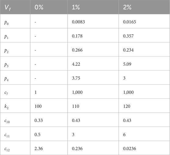
Table 3. Parameter calibration of carbon steel fiber reinforced concrete.

Figure 8

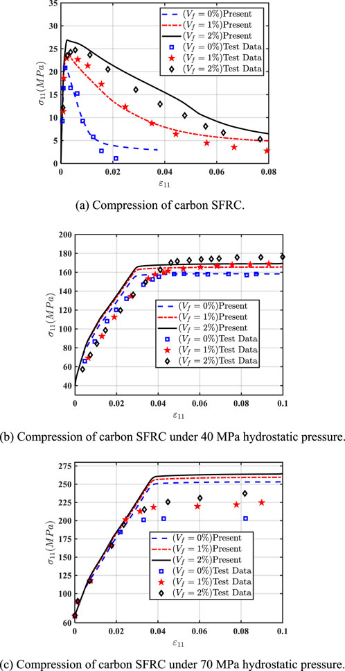
Figure 8. Experiment and simulation of carbon SFRC. (A) Compression of carbon SFRC. (B) Compression of carbon SFRC under 40 MPa hydrostatic pressure. (C) Compression of carbon SFRC under 70 MPa hydrostatic pressure.

5 Fatigue damage analysis

5.1 Plain concrete material

In this section, we consider a notched plain concrete beam of depth $D=107.8\text{mm}$, span $S=2.5D$, and a notch of length $a_0=D/6$ situated at the center of the beam. The width of the beam is $38.1\text{mm}$, as illustrated in Figure 9A. The parameters of plain concrete material: Young’s modulus $E=38.3\text{GPa}$, Poisson’s ratio $\nu =0.18$, compressive strength $f_c=90.3\text{MPa}$,density $\rho =2400\text{kg}/{\mathrm{m}}^3$. The free parameters $k_1=140\times 10^{-6}$ are calibrated by matching the peak loads of monotonic load, and the default values are adopted for all other parameters. Two finite element mesh sizes were considered, i.e., $h_{\text{size}}=3\text{mm}$ and $h_{\text{size}}=5\text{mm}$, and the predicted peak loads were $5.32\text{MPa}$ and $5.22\text{MPa}$, which were in good agreement with the experimental results $5.4\text{MPa}$ (Bazant and Schell, 1993), as shown in Figure 9B. To reduce the computational cost, the finite element mesh size of the potential damage region was $5\text{mm}$ in the subsequent analysis.

Figure 9

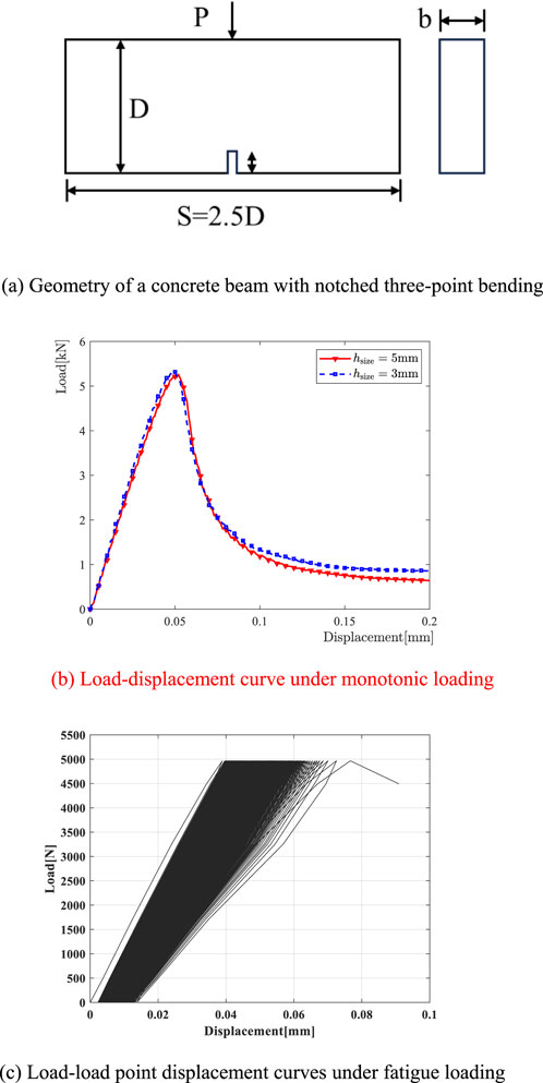
Figure 9. Simulated load-displacement curve under monotonic and fatigue loading. (A) Geometry of a concrete beam with notched three-point bending. (B) Load-displacement curve under monotonic loading. (C) Load-load point displacement curves under fatigue loading.

Next, the fatigue simulation of a three-point bending beam was performed. Cyclic loading was applied up to $84\%$ of the peak monotonic loading. The parameters of the fatigue damage law of the material are adjusted until the life prediction is satisfactorily close. The fatigue damage metric used was Equation 31, and with the adopted parameters $s=1800$ and $q=2$, the model predicted failure after 225 cycles in excellent agreement with the tested fatigue life of 212 cycles. In the last cycle, the failure is characterized by a sudden increase in the overall deformation, as shown in Figure 9C.

5.2 Steel fiber-reinforced concrete material

Then, the fatigue damage behavior of steel fiber-reinforced concrete is analyzed. A three-point bending beam (Qing et al., 2023) with notched specimen size $440\times 100\times 100\left(\mathrm{m}{\mathrm{m}}^3\right)$, a notch of width $4\text{mm}$ is located at the bottom of the middle of the beam, the height of the notch is $40\text{mm}$, and the span at the bottom of the beam is $400\text{mm}$. Four groups of steel fiber-reinforced concrete (SFRC) with steel fiber volume admixture $V_{\mathrm{f}}=0\%$, $0.5\%$, $1.0\%$, and $1.5\%$ were used. Fiber-reinforced concrete material parameters: elastic modulus $E_0=27.738\text{GPa}$, Poisson’s ratio $\nu =0.18$, tensile strength $f_t=2.67\text{MPa}$, compressive strength $f_c=34.39\text{MPa}$. The model’s free, fixed, and fiber parameters were calibrated, and the calibrated parameters are shown in Table 4. The peak monotonic loading predicted by the model is similar to the test, as shown in Table 5. The load capacity of the concrete beams was enhanced with the increase in the volume admixture of fiber-reinforced concrete.

Table 4

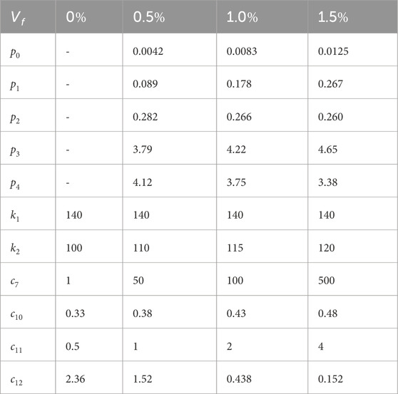
Table 4. Parameter calibration of steel fiber reinforced concrete.

Table 5

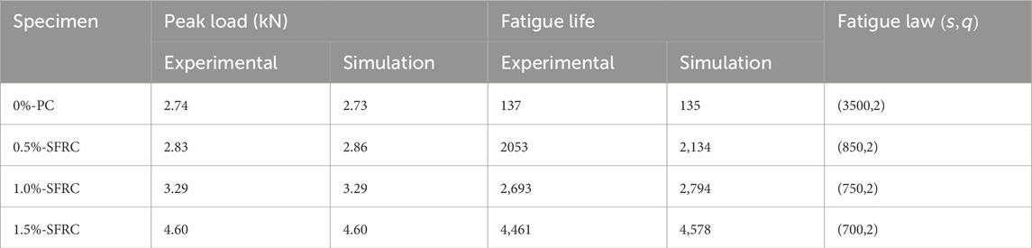
Table 5. Experiments and simulations of monotonic and fatigue loading of steel fiber reinforced concrete.

Next, fatigue analysis of fiber-reinforced concrete three-point bending beams was performed. The maximum applied cyclic load was 85% of the monotonically loaded peak load. The fatigue damage law parameters were adjusted until the life prediction was close enough. The strains of SFRC three-point bending beam with 0.5% volume steel fiber admixture for the one cycle before fatigue loading failure are shown in Figure 10A, and the strains for the remaining three groups are similar. The fatigue damage metric used is Equation 31, and the calibrated fatigue damage law parameters are shown in Table 5 for various fiber-reinforced concretes. The corresponding material fatigue damage law is shown in Figure 10B. The fatigue resistance of concrete is gradually improved with the increase of steel fiber mixing, and the fatigue resistance improvement is gradually slowed down when the steel fiber admixture is more than 1%. Therefore, the present model can be well used to analyze the mechanical response of fiber-reinforced concrete under monotonic and fatigue loading.

Figure 10

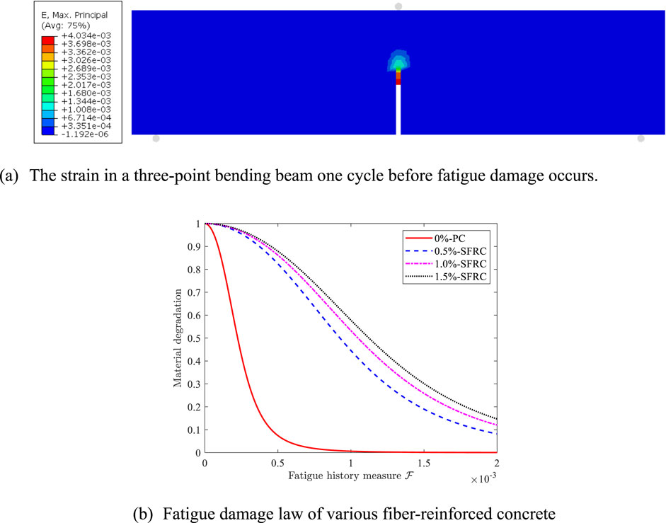
Figure 10. The strain in a three-point bending beam and fatigue damage law. (A) The strain in a three-point bending beam one cycle before fatigue damage occurs. (B) Fatigue damage law of various fiber-reinforced concrete.

5.3 Plain and steel fiber-reinforced concrete beam

Fatigue damage modeling ultimately aims to fine-tune the analysis of the whole process of fatigue damage in concrete structures. This section simulates the fatigue damage of reinforced concrete beams using the proposed model as an illustrative study. The cross-section height of the concrete beam is $h=400\text{mm}$, the cross-section width is $b=300\text{mm}$, the protective layer thickness of the steel reinforcement is $40\text{mm}$, and the cross-section reinforcement ratio of the longitudinal reinforcement $\rho \approx 1.26\%$. The geometry and loading of the concrete beam are shown in Figure 11. To show the potential of the model for capturing the fatigue damage behaviors of reinforced concrete structures, the steel reinforcement is assumed to be ideally elastic-plastic with a yield strength of $f_y=400\text{MPa}$, and the material parameters of the SFRC are the same as in the previous section.

Figure 11

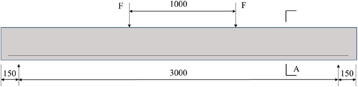
Figure 11. Geometry of reinforced concrete beams (mm) and its loaded conditions.

First, a numerical simulation of the four-point bending of reinforced concrete beams ($V_{\mathrm{f}}=0\%,0.5\%,1.0\%,1.5\%$) under monotonic loading is carried out. The load-displacement curves are shown in Figure 12. The ultimate load capacity of reinforced concrete increases gradually with the increase of fiber volume admixture, and the ultimate load capacity of reinforced concrete beams with a fiber volume admixture of 1% is the largest. Unlike the damage mechanics intrinsic model, the fatigue damage of a structure is usually accounted for by the development of strain in the microplane theory. It is worth noting that the bottom strain of plain reinforced concrete beams reaches up to 0.4361% at a displacement loading of 3 mm, and the stressed portion of the tensile zone gradually changes from concrete to steel reinforcement, as shown in Figure 13. With the increase in fiber volume admixture $V_{\mathrm{f}}=0.5\%,1.0\%,1.5\%$, the maximum strains of the resinforced concrete beams were reduced to 0.2315%, 0.0927%, and 0.065% with displacement loading of 3 m. At a displacement loading of 7.5 mm, the steel reinforcement basically stressed the tensile zone of the concrete beams, and there were some areas where the strains were close to or more than 1%. However, the concrete structure would not be subjected to such large deformations under service conditions. Afterward, we will pay attention to the response of the concrete when cracked or just cracked. In this paper, the load capacity corresponding to a plain reinforced concrete beam subjected to a displacement loading of 3 mm is defined as $F_{\mathrm{u}}=124.72\text{kN}$, and the maximum value of the fatigue load magnitude is $0.9F_{\mathrm{u}}$.

Figure 12

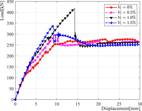
Figure 12. Load-displacement curves of reinforced concrete beams under monotonic loading ($V_{\mathrm{f}}=0\%,0.5\%,1\%,1.5\%$).

Figure 13

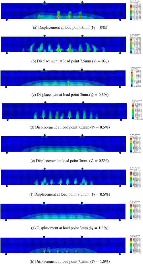
Figure 13. Strain in reinforced concrete beams under monotonic loading. (A) Displacement at load point 3 mm ($V_{\mathrm{f}}=0\%$). (B) Displacement at load point 7.5 mm ($V_{\mathrm{f}}=0\%$). (C) Displacement at load point 3 mm ($V_{\mathrm{f}}=0.5\%$). (D) Displacement at load point 7.5 mm ($V_{\mathrm{f}}=0.5\%$). (E) Displacement at load point 3 mm ($V_{\mathrm{f}}=0.5\%$). (F) Displacement at load point 7.5 mm ($V_{\mathrm{f}}=0.5\%$). (G) Displacement at load point 3 mm ($V_{\mathrm{f}}=1.5\%$). (H) Displacement at load point 7.5 mm ($V_{\mathrm{f}}=1.5\%$).

Next, fatigue damage simulations of reinforced concrete structures ($V_{\mathrm{f}}=0\%,0.5\%,1\%,1.5\%$) under 200 cyclic loadings were performed. During cyclic loading, the fatigue history variables are gradually accumulated, resulting in gradual degradation of the material stiffness and gradual development of the strain in the concrete beams. The strain distribution after 200 loading cycles is shown in Figure 14. For a reinforced concrete beam composed of plain concrete with a fatigue life of 176 cyclic loadings, the strains at one time before structural failure are shown in Figure 14A. The strains at the bottom of the beam are more than 1% in most regions. With the increase in fiber dosage, the strain of the concrete structure improved during fatigue loading due to the improvement in tensile capacity, and the cracking pattern was transformed. The beam strain distribution after 200 loading cycles is shown in Figures 14B–D. The maximum strains of reinforced concrete beams with steel fiber volume admixture $V_{\mathrm{f}}=0.5\%,1\%,1.5\%$ are 0.1313%,0.1231%, and 0.1194%, respectively. The displacements at the loading points also show a significant reduction trend, as shown in Figure 15. Therefore, the microplane model considering the material stiffness degradation can be used to reflect the fatigue damage behavior of plain and fiber-reinforced concrete materials.

Figure 14

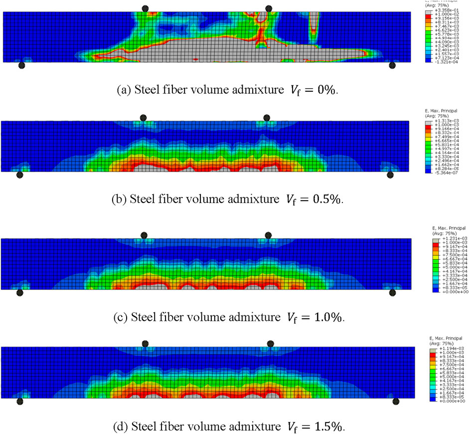
Figure 14. Reinforced concrete beam strains after fatigue loading. (A) Steel fiber volume admixture $V_{\mathrm{f}}=0\%$. (B) Steel fiber volume admixture $V_{\mathrm{f}}=0.5\%$. (C) Steel fiber volume admixture $V_{\mathrm{f}}=1.0\%$. (D) Steel fiber volume admixture $V_{\mathrm{f}}=1.5\%$.

Figure 15

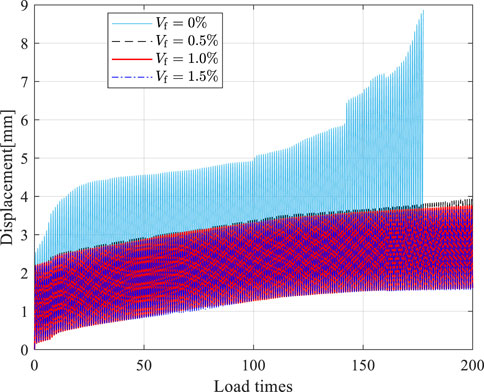
Figure 15. Displacement-loading number curves at loading point. ($V_{\mathrm{f}}=0\%,0.5\%,1\%,1.5\%$).

It is worth noting that for the fatigue of reinforced concrete structures, to capture the various mechanical behaviors in the tests, the slip between the concrete and the reinforcement also needs to be considered, and the degradation of the fatigue properties of materials such as reinforcement and fibers needs to be considered. However, this is not the focus of this study and will be illustrated in future studies. This model is expected to be used for the whole-process analysis of fatigue damage of plain concrete and steel fiber-reinforced concrete structures under complex loading conditions and structural forms, which will facilitate engineering design, evaluation, and optimization.

6 Further study

Despite the success in expanding the application of microplanar modeling of plain concrete, many issues need to be solved. In subsequent research, the following issues will be focused on:

(1) simplifying the extremely cumbersome parameters in M7 and developing user-friendly software tools or plug-ins.

(2) Consider the fatigue-related material stiffness under compression conditions and extend the model to compression fatigue analysis.

(3) Optimize the fiber toughening mechanism and expand the model to fatigue damage analysis of concrete materials such as ECC and UHPFRC.

7 Conclusion

This study successfully extends the microplane model for assessing fatigue damage in steel fiber-reinforced concrete (SFRC). The model combines material stiffness degradation, critical for analyzing fatigue damage, with fatigue history variables accumulated during cyclic loading. A more detailed prediction of the fatigue life and behavior of plain and steel fiber-reinforced concrete materials is possible. The following conclusions were obtained:

(1) The extended microplane model is suitable for mechanical response analysis of steel fiber-reinforced concrete materials. It provides an effective tool for predicting fatigue damage of concrete structures under cyclic loading by introducing fatigue history variables and establishing their relationship with material stiffness degradation.

(2) It is shown that steel fiber incorporation can substantially improve concrete’s mechanical properties and fatigue resistance. The extended model can capture the reinforcing effect of fibers, which is consistent with the experiments.

(3) The model’s parameters can be calibrated against benchmark experimental data. The model can be implemented numerically in ABAQUS commercial finite element software in conjunction with a crack band model for engineering analysis.

(4) The model can predict the fatigue life and mechanical behavior of plain and steel fiber-reinforced concrete materials, which helps in engineering design and optimization. Next, it is expected to be used for fatigue analysis of concrete structures under complex loading conditions and structural forms by considering the slip of reinforcement with concrete and the degradation of the fatigue performance of reinforcement.

Data availability statement

The original contributions presented in the study are included in the article/supplementary material, further inquiries can be directed to the corresponding author.

Author contributions

CQ: Methodology, Supervision, Writing–original draft, Writing–review and editing. XD: Funding acquisition, Resources, Writing–original draft. BW: Data curation, Investigation, Writing–original draft. LC: Validation, Visualization, Writing–original draft. SW: Formal Analysis, Project administration, Writing–original draft. QX: Conceptualization, Software, Writing–review and editing, Writing–original draft.

Funding

The author(s) declare that financial support was received for the research, authorship, and/or publication of this article. The research described in this paper was financially supported by the China Construction Third Bureau First Engineering Co., Ltd. (Grant No. CSCEC3B1C-2022-13).

Conflict of interest

Authors CQ, XD, BW, LC, and SW were employed by China Construction Third Bureau First Engineering Co., Ltd.

The remaining author declares that the research was conducted in the absence of any commercial or financial relationships that could be construed as a potential conflict of interest.

The authors declare that this study received funding from China Construction Third Bureau First Engineering Co., Ltd. The funder had the following involvement in the study: study design, data collection, funding acquisition, preparation of the paper, and decision to submit it for publication.

Generative AI statement

The author(s) declare that no Generative AI was used in the creation of this manuscript.

Publisher’s note

All claims expressed in this article are solely those of the authors and do not necessarily represent those of their affiliated organizations, or those of the publisher, the editors and the reviewers. Any product that may be evaluated in this article, or claim that may be made by its manufacturer, is not guaranteed or endorsed by the publisher.

References

Aas-Jakobsen, K. (1970). Fatigue of concrete beams and columns. Trondheim: University of Trondheim.

Google Scholar

Aguilar, M., Baktheer, A., and Chudoba, R. (2022). “Numerical investigation of load sequence effect and energy dissipation in concrete due to compressive fatigue loading using the new microplane fatigue model MS1,” in Presentations and videos to 16th International Conference on Computational Plasticity (COMPLAS 2021). IS17-Multiscale Modelling of Concrete and Concrete Structures. doi:10.23967/complas.2021.053

CrossRef Full Text | Google Scholar

Baktheer, A., Aguilar, M., and Chudoba, R. (2021). Microplane fatigue model MS1 for plain concrete under compression with damage evolution driven by cumulative inelastic shear strain. Int. J. Plasticity 143, 102950. doi:10.1016/j.ijplas.2021.102950

CrossRef Full Text | Google Scholar

Bažant, Z. P., and Oh, B. H. (1983). Crack band theory for fracture of concrete. Mat. Constr. 16, 155–177. doi:10.1007/BF02486267

CrossRef Full Text | Google Scholar

Bazant, Z. P., and Schell, W. F. (1993). Fatigue fracture of high-strength concrete and size effect. Mater. J. 90, 472–478. doi:10.14359/3880

CrossRef Full Text | Google Scholar

Bažant, Z. P., Xiang, Y., and Prat, P. C. (1996). Microplane model for concrete. I: stress-strain boundaries and finite strain. J. Eng. Mech. 122, 245–254. doi:10.1061/(ASCE)0733-9399(1996)122:3(245)

CrossRef Full Text | Google Scholar

Caner, F. C., and Bažant, Z. P. (2013a). Microplane model M7 for plain concrete. I: formulation. J. Eng. Mech. 139, 1714–1723. doi:10.1061/(ASCE)EM.1943-7889.0000570

CrossRef Full Text | Google Scholar

Caner, F. C., and Bazant, Z. P. (2013b). Microplane model M7 for plain concrete. II: calibration and verification. J. Eng. Mech. 139, 1724–1735. doi:10.1061/(ASCE)EM.1943-7889.0000571

CrossRef Full Text | Google Scholar

Caner, F. C., Bažant, Z. P., and Wendner, R. (2013). Microplane model M7f for fiber reinforced concrete. Eng. Fract. Mech. 105, 41–57. doi:10.1016/j.engfracmech.2013.03.029

CrossRef Full Text | Google Scholar

Carlesso, D. M., de la Fuente, A., and Cavalaro, S. H. P. (2019). Fatigue of cracked high performance fiber reinforced concrete subjected to bending. Constr. Build. Mater. 220, 444–455. doi:10.1016/j.conbuildmat.2019.06.038

CrossRef Full Text | Google Scholar

Červenka, J., Bažant, Z. P., and Wierer, M. (2005). Equivalent localization element for crack band approach to mesh-sensitivity in microplane model. Int. J. Numer. Methods Eng. 62, 700–726. doi:10.1002/nme.1216

CrossRef Full Text | Google Scholar

Chern, J., Yang, H., and Chen, H. (1993). Behavior of steel fiber reinforced concrete in multiaxial loading. Mater. J. 89. doi:10.14359/1242

CrossRef Full Text | Google Scholar

Chu, S. H., Unluer, C., Yoo, D. Y., Sneed, L., and Kwan, A. K. H. (2023). Bond of steel reinforcing bars in self-prestressed hybrid steel fiber reinforced concrete. Eng. Struct. 291, 116390. doi:10.1016/j.engstruct.2023.116390

CrossRef Full Text | Google Scholar

Cornelissen, H. A. W. (1984). Fatigue failure of concrete in tension. HERON 29 (4), 1–68. Available at: https://www.semanticscholar.org/paper/Fatigue-Failure-of-Concrete-in-Tension-Cornelissen/660b8ce20194711cb9477f0f6fc30503c637af43 (Accessed June 25, 2023).

Google Scholar

Gylltoft, K. (1984). A fracture mechanics model for fatigue in concrete. Mat. Constr. 17, 55–58. doi:10.1007/BF02474057

CrossRef Full Text | Google Scholar

Hillerborg, A., Modéer, M., and Petersson, P.-E. (1976). Analysis of crack formation and crack growth in concrete by means of fracture mechanics and finite elements. Cem. Concr. Res. 6, 773–781. doi:10.1016/0008-8846(76)90007-7

CrossRef Full Text | Google Scholar

Huang, B.-T., Zhu, J.-X., Weng, K.-F., Li, V. C., and Dai, J.-G. (2022). Ultra-high-strength engineered/strain-hardening cementitious composites (ECC/SHCC): material design and effect of fiber hybridization. Cem. Concr. Compos. 129, 104464. doi:10.1016/j.cemconcomp.2022.104464

CrossRef Full Text | Google Scholar

Jiang, J., Luo, Q., Wang, F., Sun, G., and Liu, Z. (2023). Uniaxial tensile constitutive model of fiber reinforced concrete considering bridging effect and its numerical algorithm. J. Sustain. Cement-Based Mater. 12, 207–217. doi:10.1080/21650373.2022.2034549

CrossRef Full Text | Google Scholar

Kholmyansky, M. M. (2002). Mechanical resistance of steel fiber reinforced concrete to axial load. J. Mater. Civ. Eng. 14, 311–319. doi:10.1061/(ASCE)0899-1561(2002)14:4(311)

CrossRef Full Text | Google Scholar

Kirane, K., and Bažant, Z. P. (2015). Microplane damage model for fatigue of quasibrittle materials: sub-critical crack growth, lifetime and residual strength. Int. J. Fatigue 70, 93–105. doi:10.1016/j.ijfatigue.2014.08.012

CrossRef Full Text | Google Scholar

Lakavath, C., Prakash, S. S., and Allena, S. (2024). Tensile characteristics of ultra-high-performance fibre-reinforced concrete with and without longitudinal steel rebars. Mag. Concr. Res. 76, 738–754. doi:10.1680/jmacr.23.00181

CrossRef Full Text | Google Scholar

Li, B., Chen, Z., Wang, S., and Xu, L. (2024). A review on the damage behavior and constitutive model of fiber reinforced concrete at ambient temperature. Constr. Build. Mater. 412, 134919. doi:10.1016/j.conbuildmat.2024.134919

CrossRef Full Text | Google Scholar

Li, B., Chi, Y., Xu, L., Li, C., and Shi, Y. (2018). Cyclic tensile behavior of SFRC: experimental research and analytical model. Constr. Build. Mater. 190, 1236–1250. doi:10.1016/j.conbuildmat.2018.09.140

CrossRef Full Text | Google Scholar

Lu, C., Leung, C. K. Y., and Li, V. C. (2017). Numerical model on the stress field and multiple cracking behavior of Engineered Cementitious Composites (ECC). Constr. Build. Mater. 133, 118–127. doi:10.1016/j.conbuildmat.2016.12.033

CrossRef Full Text | Google Scholar

Marigo, J. J. (1985). Modelling of brittle and fatigue damage for elastic material by growth of microvoids. Eng. Fract. Mech. 21, 861–874. doi:10.1016/0013-7944(85)90093-1

CrossRef Full Text | Google Scholar

Miarka, P., Seitl, S., Bílek, V., and Cifuentes, H. (2022). Assessment of fatigue resistance of concrete: S-N curves to the Paris’ law curves. Constr. Build. Mater. 341, 127811. doi:10.1016/j.conbuildmat.2022.127811

CrossRef Full Text | Google Scholar

Nguyen, D.-L., Le, H.-V., Vu, T.-B.-N., Nguyen, V.-T., and Tran, N.-T. (2023). Evaluating fracture characteristics of ultra-high-performance fiber-reinforced concrete in flexure and tension with size impact. Constr. Build. Mater. 382, 131224. doi:10.1016/j.conbuildmat.2023.131224

CrossRef Full Text | Google Scholar

Paris, P., and Erdogan, F. (1963). A critical analysis of crack propagation laws. J. Basic Eng. 85, 528–533. doi:10.1115/1.3656900

CrossRef Full Text | Google Scholar

Qing, L., Wang, Y., Li, M., and Mu, R. (2023). Fatigue life and fracture behaviors of aligned steel fiber reinforced cementitious composites (ASFRC). Int. J. Fatigue 172, 107643. doi:10.1016/j.ijfatigue.2023.107643

CrossRef Full Text | Google Scholar

Riyar, R. L., Mansi, M., and Bhowmik, S. (2023). Fatigue behaviour of plain and reinforced concrete: a systematic review. Theor. Appl. Fract. Mech. 125, 103867. doi:10.1016/j.tafmec.2023.103867

CrossRef Full Text | Google Scholar

Wille, K., El-Tawil, S., and Naaman, A. E. (2014). Properties of strain hardening ultra high performance fiber reinforced concrete (UHP-FRC) under direct tensile loading. Cem. Concr. Compos. 48, 53–66. doi:10.1016/j.cemconcomp.2013.12.015

CrossRef Full Text | Google Scholar

Yoo, D.-Y., Kim, S., Park, G.-J., Park, J.-J., and Kim, S.-W. (2017). Effects of fiber shape, aspect ratio, and volume fraction on flexural behavior of ultra-high-performance fiber-reinforced cement composites. Compos. Struct. 174, 375–388. doi:10.1016/j.compstruct.2017.04.069

CrossRef Full Text | Google Scholar

Zhang, H., Chen, S., Zhang, W., and Liu, X. (2024). Service life evaluation of curved intercity rail bridges based on fatigue failure. Infrastructures 9, 139. doi:10.3390/infrastructures9090139

CrossRef Full Text | Google Scholar

Zhu, B., Pan, J., Zhang, M., and Leung, C. K. Y. (2022). Predicting the strain-hardening behaviour of polyethylene fibre reinforced engineered cementitious composites accounting for fibre-matrix interaction. Cem. Concr. Compos. 134, 104770. doi:10.1016/j.cemconcomp.2022.104770

CrossRef Full Text | Google Scholar