Modeling moist air effects and shape memory alloys in elastocaloric devices

Elastocaloric systems, which leverage shape memory alloys (SMAs) to achieve efficient, eco-friendly thermal management, offer a promising alternative to conventional air conditioning technologies. This study presents a simulation-based approach to modeling the effects of moist air and condensation phenomena within these systems. Here, we examine key factors affecting SMA performance, including mechanical behavior and the material’s latent heat characteristics. Moist air, particularly under conditions where temperatures fall below the dew point, introduces condensation and latent heat release, which can influence thermal output in elastocaloric systems. This work develops a comprehensive model that couples the thermomechanical behavior of SMAs with the thermodynamics of moist air, incorporating condensation heat transfer, mass balance, and moisture transport. Through simulations, we quantify the impact of condensation on device level and assess how ambient moisture conditions affect overall heat exchange. The findings enhance our understanding of elastocaloric system performance under real-world conditions, contributing to the advancement of sustainable and modern technologies.

1 Introduction

Elastocaloric (EC) materials have received considerable attention from researchers and industry recently for their potential utilization in air conditioning technologies. These materials, typically SMAs such as binary Nitinol (Ni-Ti), exhibit a significant temperature change when subjected to mechanical stress, a phenomenon known as the elastocaloric effect. This effect is characterized by the absorption or release of latent heat during the stress-induced phase transformation between austenitic and martensitic phases. The reversible nature of this solid-state transformation enables the repeated use of EC materials in cooling cycles, positioning them as viable candidates for next-generation technologies. The EC material’s key features are high material coefficient of performance (COP) and no global warming potential (GWP) in its use (Frenzel et al., 2015). Thus, the EU Commission and the US Department of Energy declared this technology as the most promising alternative to current vapor compression systems in 2016 (VHK and ARMINES, 2016; Goetzler et al., 2014). This unique material, originally developed for biomedical applications, already shows promising temperature differences of up to 40 K between hot and cold state, which corresponds to an adiabatic temperature change of around 20 K during loading or unloading (Frenzel et al., 2018). Elastocalorically optimized materials from early-stage research demonstrated a material COP of over 30 (Frenzel et al., 2015).

The development of elastocaloric devices has seen significant advancements since Takeuchi et al. introduced the first technological demonstrator in 2012 (Cui et al., 2012). Over the years, various system concepts and architectures have been realized in demonstration devices. In 2016, Qian et al. introduced a compression-based system using water as a heat transfer medium (Qian et al., 2016), while Tusek et al. presented the first regenerative tensile-loaded elastocaloric system (Tušek et al., 2016). Approaches utilizing thin metal foils for heat transfer via physical contact were proposed by Ossmer et al. (2016) and Bruederlin et al. (2018). That same year, Saarland University developed the first demonstrator capable of continuously cooling air directly without an additional heat exchange medium, as part of the German Research Foundation (DFG) Priority Program SPP 1599 “Ferroic Cooling” (Welsch et al., 2018a). In 2021, the Fraunhofer group led by Bartholomé introduced the “Active Elastocaloric Heatpipe” (AEH), combining compression-loaded elastocaloric materials with the heatpipe principle for efficient heat transfer (Bachmann et al., 2021; Ianniciello et al., 2022). More recently, in 2023, the University of Naples unveiled SUSSTAIN-EL, the first Italian rotary demonstrator for air conditioning (Borzacchiello et al., 2023; Cirillo et al., 2024). And CHECK TEMPERATURE, an electronic cooling device utilizing bending-loaded NiTi wires (Cirillo et al., 2023). Nonetheless, besides tension and compression loads, torsion load was investigated as well by Wang et al., in 2019 using twistocaloric cooling on material-level by applying torsional load on NiTi wires showing increased cooling efficiency compared to tension load (Wang et al., 2019). All these applications of EC system show that there is a high demand in international research in this topic and underlines the importance of further investigations.

The development of elastocaloric systems necessitates comprehensive modeling at both the material and system levels to optimize performance and efficiency. Material-level modeling focuses on understanding the thermomechanical behavior of SMAs including phase transformation kinetics, mechanical hysteresis and thermodynamics. Accurate models are essential for predicting the material’s response to cyclic loading and for designing materials with enhanced properties. In 1985 Achenbach and Müller presented a material model for SMAs including the thermodynamics on energy level and the kinetic theory with its microscopic properties (Achenbach and Müller, 1985). Further optimizations were done in years 1989 from Achenbach (1989) and 2001 from Müller and Seelecke (2001) resulting in the Müller, Achenbach and Seelecke (M-A-S) model, which serves until today as a baseline for material modeling of SMAs (Ballew and Seelecke, 2019).

System-level modeling, on the other hand, involves the integration of elastocaloric materials into practical cooling or heating devices. This includes the design of mechanical parts to apply and release stress, heat exchangers to manage heat transfer, and control systems to regulate the cooling or heating cycle. Numerical models simulate the performance of the entire system, accounting for factors such as heat transfer coefficients, system geometry, and operational parameters (Welsch et al., 2020; Welsch et al., 2018b).

Incorporating moisture considerations into EC system modeling is crucial for several reasons. The presence of moisture in the air can lead to condensation when the temperature in the system drops below the dew point. The latent heat released during condensation can impact the thermal dynamics of the system. Neglecting these effects may lead to inaccuracies in temperature predictions and, consequently, in the assessment of the system’s cooling capacity. Incorporating moisture-related latent heat effects into the energy balance equations ensures a more accurate representation of the system’s thermodynamics. Modeling moist air properties allows for the design of more efficient heat exchangers and the optimization of airflow rates to achieve desired cooling or heating performance. The significance of this topic plays a role in applications sensitive to environmental conditions such as in the automotive sector or in-house air conditioning.

This study presents a first approach to model condensation effects and implements EC system-level simulations. Current material and system models do not cover this phenomenon which motivates a first investigation.

In the first chapter the EC material model is explained. It covers the basic knowledge as well as in depth explanations on how to model the thermomechanical behavior of the EC material. This includes stress-strain relationship, latent heats, kinetics, and heat transfer mechanisms. In the following chapter the EC system-level model is explained followed by the Moist Air Model. This chapter is the focus of this study as it explains in detail which physics and mechanisms need to be covered in order to implement moist air effects into the model. Finally, the chapter Results and Discussion will show the simulations results, interpreting and discussing the presented figures. At the end The Summary and Outlook section will present an evaluation of the model, highlighting its strengths and limitations, along with recommendations for specific areas where further work is required.

2 Elastocaloric material model

This section describes the EC material model, which is characterized by its unique hysteretic mechanical response, considered quasi-elastic. The transformation between austenite and martensite phases occurs at different stress levels, with the gap between these stress levels defining the hysteresis width. The model also incorporates the material’s thermal response. During the austenite-to-martensite (A-M) transformation, latent heat is generated, causing the material to heat up, while the reverse martensite-to-austenite transformation (M-A) absorbs heat from the environment, leading to cooling. The model integrates these thermo-mechanical phenomena through a coupling mechanism.

2.1 Stress-strain relationship

For the EC material a constitutive equation is needed to provide the stress-strain relationship. Some assumptions are set. For a material that is a mixture of martensite and austenite, the total macroscopic strain $\epsilon$ can be expressed as the combined average strain contributions from each phase ${\epsilon }_i$ along with their respective volume fractions $x_i$ (Equation 1):

$\epsilon ={\epsilon }_A{x}_A+{\epsilon }_M{x}_M(1)$

with the condition $1=x_A+x_M$. The average strains or the phase strains are given by:

${\epsilon }_A\left(\sigma \right)=\frac{\sigma }{E_A};{\epsilon }_M\left(\sigma \right)=\frac{\sigma }{E_M}+{\epsilon }_{tr}(2)$

with the elastic moduli $E_A$ and $E_M$ and the transformation strain ${\epsilon }_{tr}$. Solving Equation 2 for stress $\sigma$ yields:

$\sigma \left(\epsilon \right)=\frac{\epsilon -{\epsilon }_{tr}{x}_M}{\frac{x_A}{E_A}+\frac{x_M}{E_M}}(3)$

Equation 3 is the stress-strain relation for the used model which functions as a simple mixture-type constitutive equation.

Additionally, the effective elastic modulus $E_{eff}$ can be related to the combination of the individual moduli, weighted by their respective volume fractions (Equation 4):

$\frac{1}{E_{eff}}=\frac{x_A}{E_A}+\frac{x_M}{E_M}(4)$

The effective elastic modulus will play a significant role modeling inner loops to account for an elastic unloading process in a mixed austenite/martensite phase state.

Experiments can be made to extract the parameters for the temperature dependency to feed the model. A standard isothermal tension load experiment can be repeated at different ambient temperatures. This way we can derive change in the transformation stress as a function of the temperature. Usually this is followed by a linearization since the working parameters are in the range of −20°C–80°C in extreme scenarios, in which the temperature dependency is almost linear (Schmidt et al., 2016). For common binary Nitinol alloys the temperature dependency of the transformation stress is around $7MPa/K$. The parameter is derived from the incremental increase of the transformation stress $d{\sigma }_a$ divided by the incremental increase in temperature $dT$ (Equation 5):

$\frac{d{\sigma }_a}{dT}=\frac{d{\sigma }_m}{dT}=\frac{d\sigma }{dT}(5)$

There can be a disparity between the temperature dependency of the AM transformation and the MA transformation. In this model for simplicity, we set them to be equal. For a given temperature we can use Equation 6 to describe the transformation stress:

${\sigma }_a\left(T\right)={\sigma }_{a,ref}+\frac{d\sigma }{dT}\left(T-T_{ref}\right)(6)$

with the reference parameter of the transformation stress ${\sigma }_{a,ref}$ of the experiment at a given temperature $T_{ref}$. This relationship holds true for the reversed transformation from martensite to austenite as well (Equation 7):

${\sigma }_m\left(T\right)={\sigma }_{m,ref}+\frac{d\sigma }{dT}\left(T-T_{ref}\right)(7)$

with the hysteresis width $∆\sigma$ (Equation 8):

$∆\sigma ={\sigma }_a\left(T\right)-{\sigma }_m\left(T\right)={\sigma }_{a,ref}-{\sigma }_{m,ref}(8)$

Here an assumption has been made to keep the temperature dependency of the austenite and martensite phase to be constant and equal.

2.2 Latent heat

The value of the latent heat released and absorbed by the material is commonly determined by either Differential Scanning Calometry (DSC) or Infrared Camera experiments (IR) (Louia et al., 2023). For simplicity we assume a constant latent heat of $H=15.6J/g$ for both forward and reverse phase transformations in the model for the given EC material.

The latent heat $H$ is a crucial material parameter. Nonetheless different strain rates in experiments do not release or absorb the same amount of energy. Experiments showed that the change in temperature of the material depends on the strain rate in a way that there is an adiabatic limit for a given material. This means an increase of the strain rate over that limit results in no further temperature increase. For an efficient EC material usage that adiabatic limit must be derived through experiments. Converting that information into the model requires the change in temperature to be dependent on the transformation rate ${\dot{x}}_M$ multiplied by $H$ (Equation 9):

$\frac{\partial T}{\partial t}\sim \frac{\partial x_M}{\partial t}H(9)$

2.3 Kinetics

The transformation probability for the transformation between the two phases austenite and martensite seeks a lot of attention.

In this study we consider the Helmholtz Free Energy (HFE) $\psi$ as a key factor to derive transition probabilities. The HFE is directly connected to the stress value as shown in Equation 10:

$\frac{d\psi }{d\epsilon }=\sigma \left(\epsilon \right)(10)$

Further the Gibbs Free Energy (GFE) $g$ considers the actual stress and strain level (Equation 11):

$g=\psi -\sigma \epsilon (11)$

Applying stress to the material will change the energy minimum of the martensite phase and thus the relative energy difference of the minima. At a certain stress level, the transformation stress ${\sigma }_a$, the minimum of the martensite energy branch reaches a level the materials driving force triggers the phase transformation. The higher the difference between the minima of the austenite and the martensite phase, the higher the probability of transforming. Additionally, the temperature dependency is modelled in way that it changes the initial minimum of the stress-free austenite phase, reaching lower values at high temperatures (more stable phase) and higher values at lower temperatures (less stable phase). Combining those effects will lead to a probability function:

$p^{\alpha \beta }=\frac{1}{\tau }{e}^{\frac{-{\Delta G}^{\alpha \beta }\left(\sigma ,T\right)V_A}{k_{B}T}}(12)$

where $\tau$ and $V_A$ are the thermal activation parameters, the sampling frequency and the activation volume respectively, $\Delta G^{\alpha \beta }$ the energy difference between minimum energy and neighboring inflection point energy and $k_B$ the Boltzmann constant. The variables $\alpha \beta$ in Equation 12 indexing the A-M transformation ($\left.\alpha =A;\beta =M\right)$ or the M-A transformation ($\left.\alpha =M;\beta =A\right)$. The detailed calculation of energy landscapes can be read in (Ballew and Seelecke, 2019).

To determine the kinetics or the transformation rate of a given transformation, we combine the thermally activated probability function with the actual volume fractions of the phases in Equations 13, 14:

$\frac{\partial x_A}{\partial t}=-x_A{·p}^{AM}+\left(1-x_A\right){·p}^{MA}(13)$

$\frac{\partial x_M}{\partial t}=-x_M{·p}^{MA}+\left(1-x_M\right){·p}^{AM}(14)$

2.4 Heat transfer

The phase transformation between austenite and martensite causes the material to release or absorb latent heat. This process generates a temperature change in the material, which must be effectively transferred to the surrounding air or fluid medium. To model energy transfer mechanisms, we focus on the convective heat transfer. The rate of heat transfer by convection depends on the convective heat transfer coefficient $h$. This coefficient is determined by the flow characteristics of the fluid around the surface of the EC material. The coefficient $h$ is influenced by fluid properties (thermal conductivity, viscosity, specific heat), fluid flow velocity (laminar, turbulent) and the surface geometry. The general equation for convective heat transfer from a surface to a fluid is given by Equation 15:

${\dot{Q}}_{conv}=hA\left(T-T_{env}\right)(15)$

where $T_{env}$ is the temperature of the sourrounding fluid.

To calculate $h$, we use dimensionless parameters like the Reynolds number $Re$, Prandtl number $\mathit{Pr}$, and Nusselt number $Nu$ along with the Churchill-Bernstein equation. The Churchill-Bernstein equation is a widely used empirical correlation for the Nusselt number for a cylinder in crossflow, but it can be adapted for other geometries (Equation 16):

$Nu=0.3+\frac{0.62{Re}^{0.5}{\mathit{Pr}}^{0.33}}{{\left(1+{\left(\frac{0.4}{\mathit{Pr}}\right)}^{0.66}\right)}^{0.25}}{\left(1+{\left(\frac{Re}{282000}\right)}^{0.625}\right)}^{0.8}(16)$

The convective heat transfer coefficient is calculated by:

$h=\frac{Nuk}{L}(17)$

where $L$ is the characterisitc length and $k$ the thermal conductivity of the fluid in Equation 17.

All thermal effects combined into one set of differential equations results in the following:

$\rho c\frac{\partial T}{\partial t}=\frac{\partial }{\partial x}\left(k\frac{\partial T}{\partial x}\right)-\frac{hA}{V}\left(T-T_{env}\right)+\frac{\partial x_M}{\partial t}H(18)$

In Equation 18 the heat conduction with the thermal conductivity $k$ can be neglected considering a homogeneous transformation behaviour of the EC material. The equation accounts for heat loss to the environment due to convection and latent heat generated or absorbed according to the kinetics.

3 Elastocaloric system simulation

The transition from modeling elastocaloric materials to simulating a complete elastocaloric system involves the integration of additional physical phenomena beyond the material’s intrinsic thermomechanical behavior. In particular, airflow dynamics play a crucial role in the overall system performance, as the air acts as a heat transfer medium between the elastocaloric material and its surroundings. To accurately capture this interaction, an additional set of governing equations is required to model the energy and mass transfer within the airflow. System-level simulations incorporate an air energy balance that accounts for heat conduction, advection and convection effects. The temperature evolution of the air $T_{air}$ is governed by an energy balance of the form:

${\rho }_{air}{c}_{air}\frac{\partial T_{air}}{\partial t}=\frac{\partial }{\partial x}\left(k_{air}\frac{\partial T_{air}}{\partial x}\right)-{\rho }_{air}{c}_{air}{\mathit{v}}_{air}\frac{\partial T_{air}}{\partial x}-\frac{hA}{V}\left(T_{air}-T_{EC}\right)(19)$

where ${\rho }_{air}$ is the density of the air, $c_{air}$ is its specific heat capacity, $k_{air}$ is its thermal conductivity, ${\mathit{v}}_{air}$ represents the air velocity and $T_{EC}$ the temperature of the EC material for heat transfer in Equation 19.

To numerically solve the coupled energy equations of the elastocaloric system, it is necessary to discretize the continuous partial differential equations (PDEs) in both space and time. Discretization transforms the continuous temperature, velocity, and moisture fields into values at discrete points (nodes) within a computational grid. Common techniques for spatial discretization include the finite difference method (FDM), finite element method (FEM), or finite volume method (FVM). Temporal discretization is achieved using explicit or implicit time-stepping schemes. For instance, the temperature gradient $\frac{{\partial }^{2}T}{\partial x^2}$ in the conduction term is approximated using central difference schemes, while the advection term $\frac{\partial T}{\partial x}$ often employs upwind differencing to maintain numerical stability. This approach enables the efficient simulation of transient heat transfer phenomena, allowing for a detailed analysis of air-material interactions and overall system performance (Patankar, 2018). Welsch et al. (Welsch et al., 2018b) explaining in detail, how the discretization is applied, and the vectorization is handled to accurately model fluid dynamics in the EC system-level simulation.

Solving Equations 18, 19 simultaneously results in the overall EC system temperature distribution covering latent heats from the EC material and heat transfer interactions with the surrounding fluid. Figure 1 gives a schematic overview of the simulation results including discretization and energy balance of the air. It is a two-dimensional representation of the cross section of the EC system, however the calculations are based on the 1D model. With this EC system model, it is possible to perform parameter sweeps such as different fluid flow rates, varying rotation frequencies or changing the number of bundles in the system to optimize the output parameters of interest, namely, thermal powers or system COP. For example, if the fluid velocity or the rotation frequency is set too high, there is not enough time for the heat transfer to interchange temperatures resulting in a lower efficiency of the system. This optimization tool helps to find the best possible combinations of input parameters for given circumstances.

Figure 1

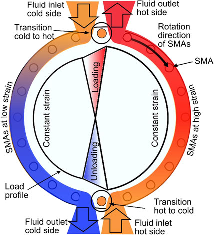
Figure 1. Schematic cross section of the temperature distribution on the fluid ducts (Welsch et al., 2018b).

This study will use the well-established EC system model to perform the simulations. A schematic machine design is shown in Figure 2. Nonetheless, another coexisting model will be implemented to cover the moist air effects and will be explained in the next section.

Figure 2

Figure 2. Schematic view of the mechanical framework for the elastocaloric device. For clarity, only eight SMA elements are shown and only one rotating disk without body is illustrated (Kirsch et al., 2017)

4 Moist air model

Moist air plays a significant role in the thermodynamic behavior of EC devices, particularly due to condensation phenomena and the release of latent heat. Understanding the fundamental properties of moist air is essential to accurately model the interaction between air, water vapor, and the EC material. This section provides an overview of key concepts such as the Mollier diagram, dew point temperature and latent heat of condensation, followed by a discussion on how these concepts can be incorporated into EC system-level simulations.

4.1 Fundamental properties

Moist air is a mixture of dry air and water vapor. The thermodynamic properties of this mixture are crucial for predicting condensation and latent heat release in elastocaloric systems.

The Mollier diagram ($h_{1+x}$ diagram) is a graphical representation of the thermodynamic properties of moist air (Figure 3). It provides relationships between the following important parameters:

• Enthalpy ($h$): Total heat content of the air-water vapor mixture (kJ/kg).

• Humidity ratio ($x$): Mass of water vapor per unit mass of dry air (kg/kg).

• Dew Point Temperature ($T_k$): The temperature at which air becomes fully saturated, leading to condensation.

Figure 3

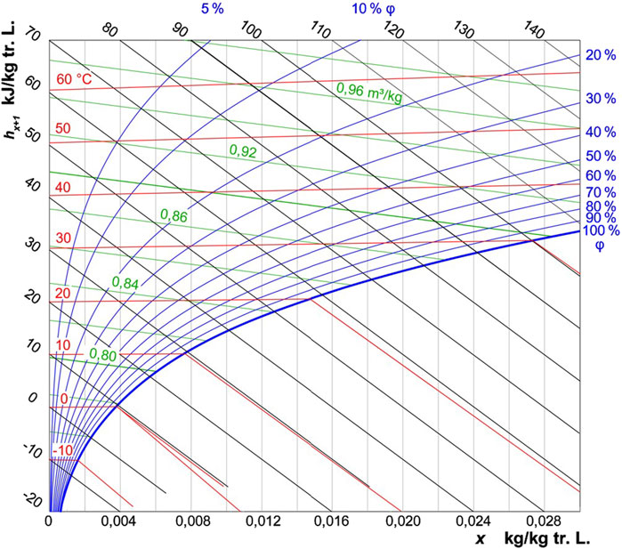
Figure 3. The Mollier diagram - specific enthalpy $h_{1+x}$ over humidity $x$; temperature in °C (red), relative humidity in % (blue) and density in m³/kg (green).

The Mollier diagram allows users to visualize how the enthalpy and humidity of air change as it cools or heats. When the air cools at constant humidity, it eventually reaches its dew point, where water vapor begins to condense. This condensation releases latent heat into the system.

4.2 Latent heat of condensation

When air cools below the dew point, water vapor condenses, releasing latent heat of condensation ($L_W$). This energy exchange is critical in elastocaloric systems where phase transitions and heat exchange with the environment occur. The released energy is given by Equation 20:

$Q_{cond}=L_W\Delta m_v(20)$

where $\Delta m_v=m_{cond}$ is the change of mass of water vapor or the mass of condensed water vapor. The release of latent heat increases the air temperature, altering the overall energy balance of the system. For simplicity we set $L_W=2500J/kg$ despite the value changes with the temperature (Koutsoyiannis, 2012).

The dew point temperature is directly related to the partial vapor pressure of water $P_v$. The partial vapor pressure can be calculated with the absolute humidity ${\phi }_{abs}$ in relation to the vapor saturation concentration ${\phi }_{\mathit{max}}$. The saturation vapor pressure $P_{sat}$ can be approximated using Clausius-Clapeyron equation or empirical Magnus-type equation (Equation 21):

$P_{sat}\left(T\right)=610.9\exp \left(\frac{17.625T}{243.04+T}\right)(21)$

with $T$ in °C and $P_{sat}\left(T\right)$ in Pa (Alduchov and Eskridge, 1996). As air cools to $T_k$, the water vapor pressure equals the saturation pressure, initiating condensation.

To quantify the mass of water vapor that condenses when the air temperature drops below the dew point, a mass balance approach is used. The key objective is to compute the amount of water vapor $\Delta m_v$ that transitions from the vapor phase to the liquid phase as a result of the temperature reduction. The calculation compares the saturation pressure $P_{sat}\left(T\right)$ with the current vapor pressure $P_v$. When the air temperature decreases below the dew point, the new saturation vapor pressure becomes lower than the current vapor pressure, causing condensation. The condensed mass of water vapor $\Delta m_v$ is calculated as by Equation 22:

$\Delta m_v=\frac{P_v-P_{sat}\left(T\right)}{R_{v}T}V=\left({\phi }_{abs}-{\phi }_{\mathit{max}}\right)V(22)$

with V the given volume and $R_v$ the specific gas constant for water vapor ($R_v=461.5J/kgK$). This approach allows for the direct calculation of condensed water vapor, which can then be used in the energy balance to account for the latent heat release associated with condensation. This fits the discretization process made for the EC system-level simulation using $V$ as the volume for a given mesh element to simultaniously and accurately align condensation calculation with the vectorization. This ensures both high spatial and time resolution results for humidity in the system.

4.3 Condensation types in the EC system

The moist air in the system can condense in different ways.

• in the air and thus fog formation

• at the chamber walls (inner and outer)

• directly on the EC material

Since the temperature must fall below the dew point, this phenomenon will only occur in the cold chamber of the EC system, which contains the cold EC material after unloading with a lower temperature than the surrounding air due to the heat transfer mechanism. This directly can lead to the assumption water droplets can form on the surface of the EC material. Model implementation wise, this means an effective heat transfer coefficient $h_{eff}$ can be used to account for the additional local parts the heat needs to be transported from the material through the water and then to the air. On top of this a certain coupling with the energy balance of the EC material needs to be done because the latent heat of condensation directly impacts the temperature of the EC material. To account for local differences in heat transfer due to the water droplets or water film formations, a possible method to calculate the effective heat transfer coefficient in this scenario could be a function to connect the value of condensed mass of water to a “loss term” which affects the actual heat transfer coefficient of the material as follows: $h_{eff}=f\left(m_{cond}\right)*h$. Nonetheless, in this dynamic system, it remains to be observed whether the effective heat transfer coefficient will significantly influence the air temperature.

Condensation as fog formation releases the latent heat directly into the air leading to a $\Delta T$. This can be implemented by changing the energy balance of the air the way that an additional term is added to account for the latent heat of the condensation upon temperature drops below dew point.

It is less likely that the water vapor will condense at the chamber walls because it is usually built out of an isolating material to minimize the heat loss from the chamber to its surroundings.

In sum, fog formation and water droplet or water film formation are both dominant mechanisms occurring in the system, which are yet in need of an experimental investigation. Possible water droplet or water film formations on the surface of the EC material and their transport in system can be avoided by implementing a brush system or air pulse blow system in the transition zones between the hot and cold sections of the real-life device.

The condensation of water as fog formation is the main objective of interest in this study and will be implemented and further explained in the next section.

4.4 Implementation in the EC system simulations

To integrate the effects of moist air into EC system-level simulations, the following thermodynamic principles are modified and applied in Equations 23-25.

1. Addition of ${\dot{q}}_{cond}$ in the energy balance of air:

$\rho c\frac{\partial T}{\partial t}={\dot{q}}_{con}+{\dot{q}}_{adv}+{\dot{q}}_{conv}+{\dot{q}}_{cond}(23)$

2. Condensation criteria; if $T<T_k$:

${m_v}^{t+1}={m_v}^t-m_{cond};Q_{cond}=L_W{m}_{cond}(24)$

3. Moisture transport:

$\frac{\partial m_v}{\partial t}=\frac{\partial }{\partial x}\left(D_v\frac{\partial m_v}{\partial x}\right)-\rho cv\frac{\partial m_v}{\partial x}-\frac{\partial m_{cond}}{\partial t}(25)$

with the diffusion coefficient of water vapor $D_v$.

The addition of ${\dot{q}}_{cond}$ accounts for the additional latent heat of condensation if temperatures fall below the dew point related to the condensation criteria.

5 Results and Discussion

This chapter presents the key results of this study and interprets their significance within the context of the research objectives. 5.1 outlines the simulation results obtained from the moist air model, while Section 5.2 provides a critical analysis of these results, highlighting their novelty and limitations.

5.1 Simulation results

While a whole parameter sweep was done, this study presents specific parameter combinations of interest. Given that a relative humidity (RH) of $30\%$ at room temperature (20°C) needs a temperature decrease of around 18°C to be saturated and considering condensation, presented results in this chapter are not focused on covering the whole parameter loops, rather than looking at specific scenarios.

In oceanic-continental climate regions relative humidities between 60% and 80% are common while temperatures may vary from around −10°C (winter) up to 30°C (summer). In this study we will cover condition combinations which seem most critical for condensation phenomena to occur as well as combinations to account for a certain critical winter case and summer case.

Table 1 shows the points of interest for a cold region including the dew point temperatures $T_{dew}$ along with the absolute and maximum humidity for the given condition. As an example: for the first parameter combination a temperature drop from 15°C to 7.3°C decreases the vapor saturation pressure equal to the actual vapor pressure initiating condensation. A further decrease in temperature leads to a higher amount of condensed water vapor covered in the simulation releasing the respective amount of energy due to the latent heat of condensation.

Table 1

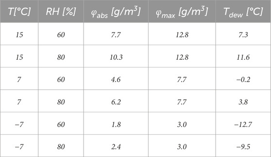
Table 1. Environmental condition combinations of interest.

As a reference EC system, we use the system-level framework presented in (Welsch et al., 2018b). It is the well-known rotatory system with equidistant bundles of EC wires aligned in the fluid chambers. For the material-level simulation a single crystal model was used, and the heat transfer medium is air. Specific material parameters can be read in (Welsch et al., 2020). Reported transformation stress values of ∼542 MPa and ∼423 MPa for ${\sigma }_a$ and ${\sigma }_m$ at room temperature respectively, motivates further investigations and optimizations made for materials used in EC devices to reduce the overall stress levels and lowering material hysteresis. A constant latent heat ($15.6J/g$) for both forward and reversed phase transformation is chosen as an average value for simplicity and computing time reasons. This results in a small error regarding the material output. The model is implemented in MATLAB and solved by a standard ode113 solver. The following system parameters were applied:

As a mid-sized EC device this set of parameters a capable of producing a temperature difference of $∆T\approx 6K$ (simulation-based) on either side of the system (hot outlet and cold outlet) while keeping, with a moderate mass of EC material used, the mechanical input relatively low. Exact values for thermal and mechanical power are not in the focus of this study and thus not explicitly mentioned. The temperature difference in each mesh element of the system seeks the attention, because the value is the key factor for the condensation criteria.

To directly match the localization of moist air simulation results with the EC system Figure 4 visualizes the EC system cross section of the parameters shown in Table 2:

Figure 4

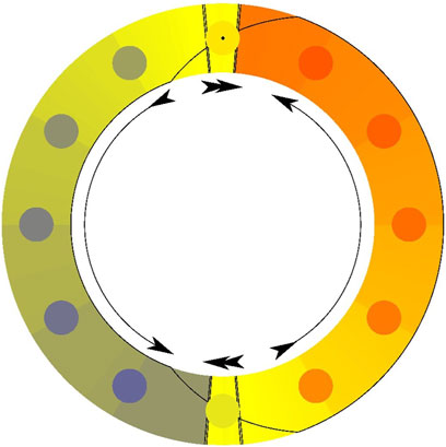
Figure 4. Schematic overview of the EC system cross section.

Table 2

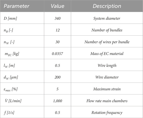
Table 2. EC system-level simulation parameters.

In Figure 4 black arrows indicating air flow direction, big dots indicating bundle location and color scaling indicating temperature distribution (qualitative). The system rotates clockwise and thus operates in counter-flow mode. Top right is the outlet of the warm side, bottom right the inlet of the warm side, top left the inlet of the cold side and bottom left the outlet of the cold side. Between both top and bottom inlets and outlets is the transition zone between warm and cold side. In these transition zones the material is mechanically loaded and unloaded indicated by the black line. The model accounts for overflow/mixing between the warm and cold sides to better represent a real-life EC system in operation. The total incoming volume flow is divided, with 83.33% directed to the main chambers and 16.66% to the transition zones. Consequently, the volume flow rates in the transition zones equal 20% of the main chamber’s volume flow rates.

The moist air simulations follow the numerical calculations as described in the previous chapters. Figure 5 shows the moist air transport in this specific EC system at an environmental temperature of 15°C and a relative humidity of 80%:

Figure 5

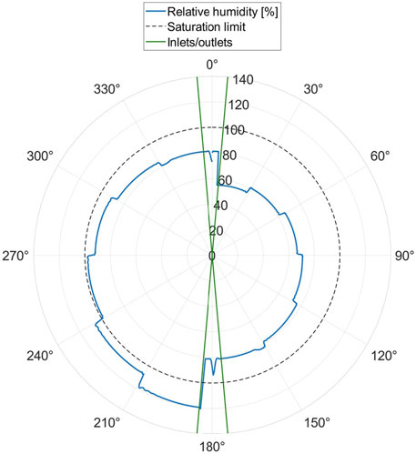
Figure 5. Simulation results; RH = 80% and $T_{in}$ = 15°C.

The results show that the temperature drop in the cold chamber triggers the condensation as expected. Once the temperature drops below the dew point temperature, condensation criteria is met.

Transported mass of water vapor plays a significant role when it comes to quantifying the effect of condensation. Table 3 summarizes the results for the given parameter sweep in Table 1 regarding moist air stream ${\dot{M}}_{moist}$ and condensate generation rate ${\dot{M}}_{cond}$.

Table 3

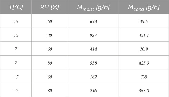
Table 3. Moist air stream and condensate generation rate.

The moist air stream represents how much water vapor will be transported throughout the system over time. This value is highly sensitive to the volume flow rate of the EC system since it directly affects heat transfer, temperature difference and moist air transport velocity. The condensation generation rate ${\dot{M}}_{cond}$ is the calculated condensed mass of water vapor over time in presented system.

Not only is the moist air transport important, but the actual temperature distribution is also a parameter of interest as well. By comparing simulation results of the same parameter combinations with completely dry air vs moist air, we assess the importance of the consideration of moist air effects in EC system-level models. As an example, the same operating parameters were applied, but the temperature of the environment is set to 30°C to account for a warmer region. Increasing the temperature from 15°C to 30°C nets a higher saturation pressure of water vapor (following Equation 21) and thus a higher absolute humidity if the relative humidity remains constant. This means the air can hold more water vapor in the gas phase exponentially. Cooling down this warm air by the same amount of $∆T$, the more water vapor will condense, resulting in a higher amount of released heat. This way we can highlight the actual difference in system performance regarding cold output with the moist air model. The temperature difference between dry air and moist air for the inlet temperature of 30°C is shown in Figure 6. Important note: the machine is already in steady state. Thus, shown results represent one rotation of the system in steady state.

Figure 6

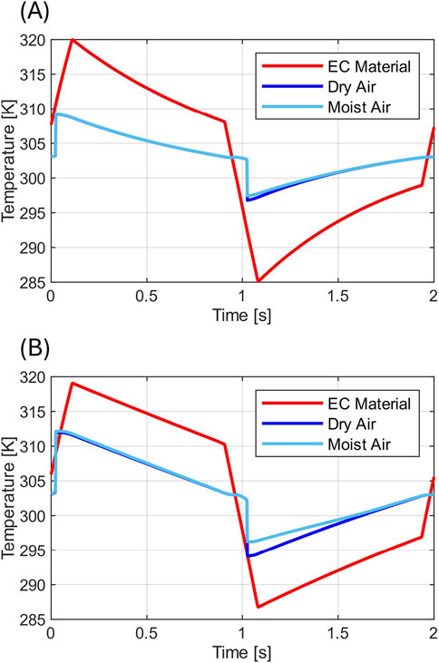
Figure 6. Comparison dry air vs moist air: temperature distribution over time for the given EC system; RH = 90% and $T_{in}$ = 30°C with (A) $\dot{V}=1000l/\mathit{min}$ and (B) $\dot{V}=500l/\mathit{min}$.

Figure 6A follows the same operating parameters as Table 2 at higher temperature. The results show the expected heat transfer between EC material and fluid. However, comparing dry air vs. moist air temperature distribution, a certain difference can be observed, which implies that the condensation in that area occurred and released its latent heat to increase the temperature of the air. The temperature of the could output changes from $T_{out,cold}^{dry}\approx 24.8°C$ to $T_{out,cold}^{moist}\approx 25.3°C$ reducing the cold output by a factor of $\sim 0.90$. In addition Figure 6B shows same results with a decrease in fluid flow rate ($\dot{V}=500l/\mathit{min}$) to increase the overall $∆T$ of the system by increasing the time to transfer the heat between the EC material and air. The temperature distribution shows a less decaying heat transfer but a slight increase in temperature output of the system. This results in a higher gap between dry and moist air since the increased temperature drop is the reason to condense more mass of water vapor. In this case the temperature of the cold output changes from $T_{out,cold}^{dry}\approx 22.5°C$ to $T_{out,cold}^{moist}\approx 24.2°C$ reducing the cold output by a factor of $\sim 0.77$. To visualize the temperature drops and resulting condensed mass of water vapor, the two cases shown in Figure 6 are added to the Mollier diagram as follows.

In Figure 7 path 1–2-3 shows how a temperature drop of $∆T=5.2K$. The thermodynamics of the moist air does not directly follow the path, indicated by the dashed black lines entering the fog region. Instead, the air reached point three by following the saturation line (100% RH) once the vertical temperature drop intersects with the saturation line. The reduction in humidity ratio $x$ of point 1 and 3 equals the actual condensed mass of water vapor for the given temperature drop. The second path 1–2′-3′ shows similar scenario with a temperature drop of $∆T=7.7K$ with higher difference on humidity ratio before and after the temperature drop (1–3′). This aligns with the temperature differences shown in Figure 6 due to the increased mass of water vapor condensing with a bigger temperature drop.

Figure 7

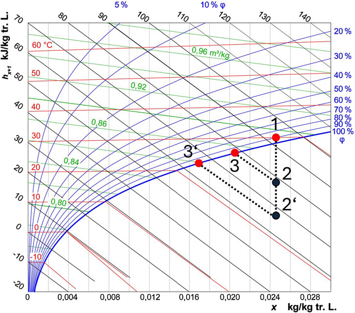
Figure 7. Simulation results shown in the Mollier diagram - connections 1-2-3 and 1–2′-3′ represent the two different scenarios.

Figure 8 provides a general overview of the impact of moist air under different ambient conditions, illustrating the expected energy loss with respect to the system’s temperature output in the cold chamber compared to dry air. Ambient temperatures of 15°C and 30°C were selected, with relative humidity levels ranging from 50% to 100%:

Figure 8

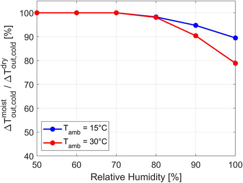
Figure 8. The effects of different ambient conditions on the thermal output of the system: 15°C (blue) and 30°C (red) at different relative humidity levels.

The key difference between the two selected ambient temperatures is the absolute humidity at a given relative humidity value. As expected, we see an increase in temperature loss for the 30°C ambient temperature due to a higher value of condensed mass of water, which leads to greater latent heat release from the condensation mechanism. For both scenarios we see the condensation phenomenon to have a considerable effect on the system starting between 70% and 80% relative humidity, reducing the efficiency by a factor of up to ∼0.89 and ∼0.79 at 100% RH (fully saturated moist air in the inlets) for 15°C and 30°C respectively. Since the system’s thermal power is directly correlated with the temperature difference between inlets and outlets of the system, those values are expected to show similar trends. The volume flow rate was set to $1000l/\mathit{min}$. The results demonstrate the impact of different ambient conditions on the EC system on heat loss and thus thermal power output.

5.2 Discussion

The simulations reveal significant insights into the moist air dynamics. This section discusses these results considering moist air transport and condensation in the EC system.

Both the inlet for the air in the warm chamber at an angle of 175° and the inlet for the air in the cold chamber at an angle of 355° have the input parameters of Table 1. Following the air flow of the warm chamber from an angle of 175°–5°, we see a steady decrease in relative humidity which is connected to the increasing temperature of air due to the heat transfer from the incoming loaded EC material releasing its latent heat. This means we see an increase in temperature along with a decrease of relative humidity. The absolute humidity ${\phi }_{abs}$ remains constant because no condensation occurs in this chamber. The heated-up air in the outlet is considered dry due to the low relative humidity. In contrast to the warm chamber, the cold chamber does reveal more interesting results. With the air incoming at an angle of 355° the moist air steadily increases in relative humidity because the incoming unloaded EC material at the angle of 185° absorbs heat from the environment, resulting in a temperature decrease of the air. In the simulation for incoming air with a relative humidity of 80% at 15°C, we see that the condensation is triggered shortly before the air reaches the outlet of the cold chamber. The combination of multiple factors influences both temperature and water vapor content in these mesh elements. The constant air flow transports moisture and is responsible for the temperature gradient in the chamber. In each element containing the EC material a certain heat exchange directly happens which decreases the temperature of the moving air. This results in a step wise temperature decrease passing bundle per bundle. Thus, the relative humidity in the cold chamber shows similar trend due to the direct connection to temperature. The moment the vapor saturation is reached, condensation criteria is met and the latent heat of condensation additionally affects the surrounding air temperature. This phenomenon is accounted for as described by Equation 23. Relative humidity values above 100% only represent the difference in current humidity and maximum possible humidity (Equation 21) to calculate how much mass of water vapor condenses. A direct drop of current humidity due to condensation is not present in the results because the air flow constantly transports water vapor between mesh elements (Equation 25). The outcoming moist air of the cold chamber is mostly saturated, which is an important criterion for specific applications. The air then mixes with the concurrent air present on the application, increasing the overall humidity.

With the results shown condensation will likely occur for specific environmental conditions. Nonetheless Table 3 summarizes how much water vapor is transported over time. This includes the moist air stream solely from the air velocity and transportation of water vapor, and the condensation generation rate covering the condensed mass of water vapor over time. The sum of both values results in the overall moist air stream coming out of the EC system. Comparing these results with the moist air stream of around $500g/h$ of a standard air conditioner with similar performance, the results show promising accuracy of the model. Gravitational effects were intentionally neglected in this study. Given the used airflow velocities of 500–1,000 $l/\mathit{min}$, the air transport terms in the energy balance are significantly more dominant than any gravitational influence on moist air movement or transport. For gravitational effects to have a meaningful impact relative to the air velocity, the airflow would need to be reduced to levels so low that no EC system could operate efficiently or effectively.

The temperature analysis reveals important and interesting results. Looking specifically at the warm region case to exploit higher absolute humidity shows significant differences between dry air and moist air in the model. As the cold side is capable of cooling down the air below dew point, the latent heat of condensation is responsible for the change in temperature outputs of the cold outlet. The results show the significance of the moist air model pointing out that considering moist air effects will change EC system-level designs to account for condensation phenomena.

Moist air physics includes both condensation and evaporation mechanisms. While this study focused on the condensation part, evaporation was not included in the model.

6 Summary and outlook

This study presents a model to account for moist air dynamics for EC systems based on mass balance and condensation criteria. While the model has not yet been validated with experimental data, it helps to address discrepancies between experimental results and simulations from existing system-level models that neglect moist air effects. Every real-life system is exposed to environmental conditions even if they are less present in specific scenarios.

The primary goal of this work is to characterize and model moist air dynamics and condensation effects. A deeper optimization of both material-level and system-level models was not done. The results serve as a baseline for future EC device development, particularly for replacing less efficient and outdated technologies.

Applications sensitive to changing environmental conditions require a deeper understanding of how temperature or humidity affects the system. Future work should focus on validating the model using controlled experiments to refine parameters and ensure alignment with experimental data. These experiments should carefully control humidity and temperature and incorporate detailed observations of condensation phenomena, such as water droplets and layers, to capture localized heat transfer variations accurately. Further parameter studies will be done to account for the sensitivity of the system to fluid flow rate, relative humidities and temperature of incoming air. Furthermore, a deeper analysis of winter cases (−10°C–10°C) and summer cases (25°C–45°C) will be done to cover a broad spectrum of possible application scenarios.

The material used for this simulative study is currently the only EC material available in large quantities for building devices. With the high transformation stress levels in this tension case, it is not expected to show sufficient lifetime cycles. Partial loading, rather than full transformation, could help to extend the material’s lifetime. However, the drawback is a reduced latent heat output. Future studies should also focus on comparing new materials, particularly those optimized for EC applications. Additionally, experimental characterization should be performed to extract key parameters for the simulations.

Data availability statement

The datasets presented in this article are not readily available because Confidential. Requests to access the datasets should be directed to DZ, ZGF2aWQuemltbWVybWFubkB1bmktc2FhcmxhbmQuZGU=.

Author contributions

DZ: Writing–original draft, Writing–review and editing. FL: Data curation, Resources, Writing–review and editing. FW: Data curation, Resources, Software, Writing–review and editing. PM: Project administration, Resources, Supervision, Writing–review and editing. SS: Conceptualization, Project administration, Resources, Supervision, Writing–review and editing.

Funding

The author(s) declare that no financial support was received for the research, authorship, and/or publication of this article.

Acknowledgments

The authors are grateful to Felix Welsch from the Intelligent Materials Systems Lab for their previous work on EC modeling and for continuous help and guidance. The authors acknowledge the use of OpenAI’s ChatGPT for language editing of this manuscript.

Conflict of interest

The authors declare that the research was conducted in the absence of any commercial or financial relationships that could be construed as a potential conflict of interest.

Generative AI statement

The authors declare that Gen AI was used in the creation of this manuscript. OpenAI’s GPT-4.

Publisher’s note

All claims expressed in this article are solely those of the authors and do not necessarily represent those of their affiliated organizations, or those of the publisher, the editors and the reviewers. Any product that may be evaluated in this article, or claim that may be made by its manufacturer, is not guaranteed or endorsed by the publisher.

References

Achenbach, M. (1989). A model for an alloy with shape memory. Int. J. Plasticity 5 (4), 371–395. doi:10.1016/0749-6419(89)90023-5

CrossRef Full Text | Google Scholar

Achenbach, M., and Müller, I. (1985). Simulation of material behaviour of alloys with shape memory. Arch. Mech. Stosow. 37 (6), 573–585.

Google Scholar

Alduchov, O. A., and Eskridge, R. E. (1996). Improved Magnus form approximation of saturation vapor pressure. J. Appl. Meteorology (1988-2005) 1, 601–609. doi:10.1175/1520-0450(1996)035<0601:imfaos>2.0.co;2

CrossRef Full Text | Google Scholar

Bachmann, N., Fitger, A., Maier, L. M., Mahlke, A., Schäfer-Welsen, O., Koch, T., et al. (2021). Long-term stable compressive elastocaloric cooling system with latent heat transfer. Commun. Phys. 4 (1), 194. doi:10.1038/s42005-021-00697-y

CrossRef Full Text | Google Scholar

Ballew, W., and Seelecke, S. (2019). Mesoscopic free energy as a framework for modeling shape memory alloys. J. Intelligent Material Syst. Struct. 30 (13), 1969–2012. doi:10.1177/1045389x19844330

CrossRef Full Text | Google Scholar

Borzacchiello, A., Cirillo, L., Greco, A., and Masselli, C. (2023). A comparison between different materials with elastocaloric effect for a rotary cooling prototype. Appl. Therm. Eng. 235, 121344. doi:10.1016/j.applthermaleng.2023.121344

CrossRef Full Text | Google Scholar

Bruederlin, F., Bumke, L., Chluba, C., Ossmer, H., Quandt, E., and Kohl, M. (2018). Elastocaloric cooling on the miniature scale: a review on materials and device engineering. Energy Technol. 6 (8), 1588–1604. doi:10.1002/ente.201800137

CrossRef Full Text | Google Scholar

Cirillo, L., Greco, A., and Masselli, C. (2023). Development of an electronic circuit cooling system using elastocaloric effect: a FEM comparison among different configurations. Appl. Therm. Eng. 219, 119463. doi:10.1016/j.applthermaleng.2022.119463

CrossRef Full Text | Google Scholar

Cirillo, L., Greco, A., and Masselli, C. (2024). The energy performances of an elastocaloric device for air conditioning through numerical investigation. Appl. Therm. Eng. 236, 121517. doi:10.1016/j.applthermaleng.2023.121517

CrossRef Full Text | Google Scholar

Cui, J., Wu, Y., Muehlbauer, J., Hwang, Y., Radermacher, R., Fackler, S., et al. (2012). Demonstration of high efficiency elastocaloric cooling with large ΔT using NiTi wires. Appl. Phys. Lett. 101 (7), 073904. doi:10.1063/1.4746257

CrossRef Full Text | Google Scholar

Frenzel, J., Eggeler, G., Quandt, E., Seelecke, S., and Kohl, M. (2018). High-performance elastocaloric materials for the engineering of bulk-and micro-cooling devices. MRS Bull. 43 (4), 280–284. doi:10.1557/mrs.2018.67

CrossRef Full Text | Google Scholar

Frenzel, J., Wieczorek, A., Opahle, I., Maaß, B., Drautz, R., and Eggeler, G. (2015). On the effect of alloy composition on martensite start temperatures and latent heats in Ni–Ti-based shape memory alloys. Acta Mater. 90, 213–231. doi:10.1016/j.actamat.2015.02.029

CrossRef Full Text | Google Scholar

Goetzler, W., Zogg, R., Young, J., and Johnson, C. (2014). Energy savings potential and RD&D opportunities for non-vapor-compression HVAC technologies. United States :Navigant Consulting Inc., prepared for US Department of Energy, 199.

Google Scholar

Ianniciello, L., Bartholomé, K., Fitger, A., and Engelbrecht, K. (2022). Long life elastocaloric regenerator operating under compression. Appl. Therm. Eng. 202, 117838. doi:10.1016/j.applthermaleng.2021.117838

CrossRef Full Text | Google Scholar

Kirsch, S. M., Schmidt, M., Welsch, F., Michaelis, N., Schütze, A., and Seelecke, S. (2017). Development of a shape memory based air conditioning system. Univ. Ilmenau.

Google Scholar

Koutsoyiannis, D. (2012). Clausius–Clapeyron equation and saturation vapour pressure: simple theory reconciled with practice. Eur. J. Phys. 33 (2), 295–305. doi:10.1088/0143-0807/33/2/295

CrossRef Full Text | Google Scholar

Louia, F., Michaelis, N., Schütze, A., Seelecke, S., and Motzki, P. (2023). A unified approach to thermo-mechano-caloric-characterization of elastocaloric materials. J. Phys. Energy 5 (4), 045014. doi:10.1088/2515-7655/acfb39

CrossRef Full Text | Google Scholar

Müller, I., and Seelecke, S. (2001). Thermodynamic aspects of shape memory alloys. Math. Comput. Model. 34 (12-13), 1307–1355. doi:10.1016/s0895-7177(01)00134-0

CrossRef Full Text | Google Scholar

Ossmer, H., Wendler, F., Gueltig, M., Lambrecht, F., Miyazaki, S., and Kohl, M. (2016). Energy-efficient miniature-scale heat pumping based on shape memory alloys. Smart Mater. Struct. 25 (8), 085037. doi:10.1088/0964-1726/25/8/085037

CrossRef Full Text | Google Scholar

Patankar, S. (2018). Numerical heat transfer and fluid flow. Boca Raton:CRC Press.

CrossRef Full Text | Google Scholar

Qian, S., Geng, Y., Wang, Y., Muehlbauer, J., Ling, J., Hwang, Y., et al. (2016). Design of a hydraulically driven compressive elastocaloric cooling system. Sci. Technol. Built Environ. 22 (5), 500–506. doi:10.1080/23744731.2016.1171630

CrossRef Full Text | Google Scholar

Schmidt, M., Ullrich, J., Wieczorek, A., Frenzel, J., Eggeler, G., Schütze, A., et al. (2016). Experimental methods for investigation of shape memory based elastocaloric cooling processes and model validation. JoVE J. Vis. Exp. 2 (111), e53626. doi:10.3791/53626-v

CrossRef Full Text | Google Scholar

Tušek, J., Engelbrecht, K., Eriksen, D., Dall’Olio, S., Tušek, J., and Pryds, N. (2016). A regenerative elastocaloric heat pump. Nat. Energy 1 (10), 16134–16136. doi:10.1038/nenergy.2016.134

CrossRef Full Text | Google Scholar

VHK and ARMINES (2016). Commision Regulation (EC) No. 643/2009 with regard to ecodesign requirements for household refrigeration appliances and Commission Delegated Regulation (EU) No. 1060/2010 with regard to energy labelling of household refrigeration appliances. Available online at: https://www.eup-network.de/fileadmin/user_upload/Household_Refrigeration_Review_TECHNOLOGY_ROADMAP_FINAL_20160304.pdf.

Google Scholar

Wang, R., Fang, S., Xiao, Y., Gao, E., Jiang, N., Li, Y., et al. (2019). Torsional refrigeration by twisted, coiled, and supercoiled fibers. Science 366 (6462), 216–221. doi:10.1126/science.aax6182

PubMed Abstract | CrossRef Full Text | Google Scholar

Welsch, F., Kirsch, S. M., Michaelis, N., Mandolino, M., Schütze, A., Seelecke, S., et al. (2020). System simulation of an elastocaloric heating and cooling device based on SMA. InSmart Mater. Adapt. Struct. Intelligent Syst. 84027, V001T03A005. American Society of Mechanical Engineers. doi:10.1115/SMASIS2020-2262

CrossRef Full Text | Google Scholar

Welsch, F., Kirsch, S. M., Michaelis, N., Motzki, P., Schmidt, M., Schütze, A., et al. (2018b). Elastocaloric cooling: system design, simulation, and realization. InSmart Mater. Adapt. Struct. Intelligent Syst. 51951, V002T08A005. American Society of Mechanical Engineers. doi:10.1115/SMASIS2018-7982

CrossRef Full Text | Google Scholar

Welsch, F., Kirsch, S. M., Michaelis, N., Schmidt, M., Schütze, A., and Seelecke, S. (2018a). Continuously operating elastocaloric cooling device based on shape memory alloys: development and realization.

Google Scholar