Corrosion prediction for shale gas pipelines based on Bayesian network and common cause failure analysis

Introduction: During the commissioning and operation of shale gas pipelines, multiple perforation accidents caused by internal corrosion have occurred. Research on internal corrosion probability prediction remains limited due to the complexity of its causes.

Methods: This paper establishes an internal corrosion probability prediction model for shale gas pipelines using a Bayesian network model combined with common cause failure analysis.

Results and Discussion: The model was applied to predict internal corrosion in pipelines within a shale gas field in Sichuan Province, China. The prediction results showed a 20% error margin compared to field inspection results.

1 Introduction

Shale gas, extracted from shale formations, is a significant unconventional natural gas resource typically transported via pipelines. As the scale of shale gas extraction and transportation expands, the safety and reliability of pipeline systems have become a critical issue. Statistics show that internal pipeline wall corrosion is one of the primary factors affecting pipeline safety, potentially leading to pipeline failure, leaks, or ruptures, and in severe cases, fires or explosions. Therefore, it is essential to study the corrosion issues within shale gas pipelines.

Compared to research on corrosion in conventional natural gas pipelines, studies on shale gas pipeline corrosion are relatively limited. Current research primarily focuses on CO₂ corrosion and sulfate-reducing bacteria (SRB) corrosion. For instance, Li et al. (2020) used optical microscopy, scanning electron microscopy, energy-dispersive spectroscopy, and X-ray diffraction to analyze the causes of corrosion failure in pipelines from six typical shale gas blocks in an oilfield, discussing the corrosion mechanisms. They found CO₂ corrosion in pipelines from four typical blocks. Palumbo et al. (2020) employed weight loss and electrochemical methods to study the effect of different CO₂ partial pressures on the corrosion inhibition performance of N80 carbon steel pipelines, noting that the protective layer on the metal surface became denser with increasing CO₂ partial pressure. Mohammed Nor (2013) focused on parameters affecting CO₂ corrosion flow sensitivity, including CO₂ partial pressure, pH, and temperature, and developed a corrosion model suitable for high CO₂ partial pressure environments, demonstrating that CO₂ partial pressure has the strongest effect on corrosion flow sensitivity. Yue and Wang (2018) analyzed the corrosion mechanisms in a shale gas pipeline block in Sichuan Province, China, identifying SRB as the main cause of pipeline perforation corrosion, with CO₂ and Cl⁻ accelerating the corrosion, exacerbated by erosion. Xie and Zhang (2018) studied corrosion issues in a shale gas pipeline in Sichuan Province, China, finding that the pipeline faced erosion corrosion and electrochemical corrosion, with sand content being a major controlling factor for erosion corrosion. The study also analyzed the impact of ambient and high-pressure conditions on the corrosion rates of various metals, showing that corrosion rates were higher in bacterial environments than in sterile ones, and that pressure changes also affected corrosion rates.

Once the main corrosion factors are identified, relevant methods can be used to assess the probability of pipeline corrosion. In recent years, Bayesian networks have increasingly been applied to this task. For example, Ayello et al. (2014) used a Bayesian network model to analyze the corrosion probability in crude oil pipelines, representing the causal relationships in complex systems as conditional probabilities. Meanwhile, the author employed a Bayesian network model to assess corrosion in a pipeline, successfully calculating the failure rate with limited known information, finding a 7% failure rate after about 20 years of use. Shabarchin and Tesfamariam (2016) established an internal corrosion probability model using a Bayesian network, simplifying corrosion model calculations and improving prediction accuracy. Shan et al. (2019) proposed a step-by-step approach using Bayesian networks to assess external and internal corrosion in buried oil pipelines by analyzing complex causal relationships through fault models, existing system knowledge, and expert input. Han et al. (2024) transformed the bowtie model into a bowtie-Bayesian model by means of logic mapping to further analyze the failure probability of the filling control system for aviation oil storage and transportation; Hu et al. (2023) combined the bowtie (BT) and dynamic Bayesian network (DBN) models to analyze the pipeline leakage behavior in the high-consequence area, and used the fuzzy probability and the Leaky Noisy-or Gate model to determine the a priori probability and conditional probability of the DBN model, and introduced the time dimension in the nodes of human factors and corrosion conditions for dynamic settings to obtain the time-varying characteristics of the probability of pipeline leakage and the probability of occurrence of accident consequences. Xiang and Zhou (2020) used the expectation-maximization algorithm to learn the parameters of the Dynamic Bayesian model for the reliability-based corrosion management of oil and natural gas pipelines. The application of the model on simulated and real corrosion data demonstrated the effectiveness of parameter learning and the accuracy of corrosion growth predicted by the DBN model. However, these studies primarily focus on oil or conventional natural gas pipelines, with few reports on corrosion probability prediction for shale gas pipelines.

Given this, this study aims to establish a shale gas pipeline internal corrosion probability model based on Bayesian networks, considering common cause failures. This model can predict the location and timing of pipeline corrosion, which is of great significance for analyzing the safety and reliability of shale gas pipelines.

2 Shale gas pipeline internal corrosion probability model based on Bayesian network

2.1 Basic concepts

Bayesian network is a directed acyclic graph based on graph theory and probability theory, designed to represent the dependency relationships and probability distributions among a set of random variables. This network typically consists of nodes, directed edges, and probabilities. Figure 1 illustrates a simple Bayesian network structure diagram.

Figure 1

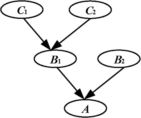
Figure 1. A simple Bayesian network structure diagram.

In the diagram, C₁, C₂, B₁, B₂, and A represent a set of random variables, with the arrows indicating the dependency relationships among these variables. C₁ is the parent node of B₁, and B₁ is the child node of C₁. C₁ and C₂, having no parent nodes, are referred to as root nodes. Root nodes have corresponding prior probability distributions, while non-root nodes have corresponding conditional probability distributions. The Bayesian network calculates the system’s failure probability using the Equation 1:

$P\left(U\right)={\displaystyle \prod _{i=1}^n}P\left(X_i/Pa\left(X_i\right)\right)(1)$

where Pa(X_i) represents the probability of the parent node X_i occurring; P(X_i/Pa(X_i)) denotes the conditional probability value of the child node occurring given that the parent node X_i has occurred; and P(U) signifies the failure probability value of the system under study.

2.2 Construction of Bayesian network structure

The construction of a Bayesian network structure primarily involves determining the network topology and, based on this, establishing the conditional probability distributions for each node. Using causal relationships to build the network structure simplifies the model and makes the probability distributions between variables easier to analyze. In this study, the No. 1 pipeline from a shale gas field in Sichuan Province, China, is used as an engineering case to construct the Bayesian network structure.

2.2.1 Node selection and variable setting

Based on field investigations, the corrosion occurring in the No. 1 pipeline primarily includes uniform corrosion, local corrosion, and SRB corrosion. The main influencing factors for each type of corrosion are listed in Table 1 below, where T represents temperature. Each influencing factor corresponds to a node in the Bayesian network.

Table 1

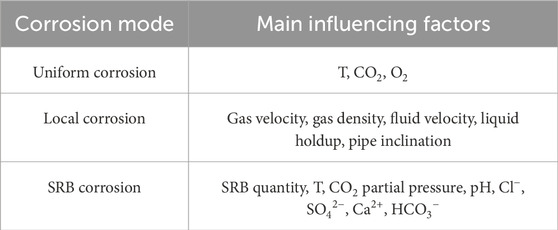
Table 1. Main influencing factors for various corrosion modes.

2.2.2 Bayesian network model

In this study, a causal relationship diagram with 38 nodes is established based on existing experience. All Bayesian network models are modeled and computed using GeNIe 2.0 software. The modeling approach employs the two-phase method, and the Bayesian network inference utilizes the variable elimination method. The Bayesian network model, constructed using data derived from expert knowledge and experiments, is illustrated in Figure 2.

Figure 2

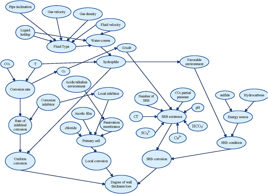
Figure 2. Bayesian network model.

2.2.3 Prior probabilities of root nodes

The prior probabilities of root nodes in a Bayesian network refer to the probabilities derived from historical statistical data or expert experience analysis. The prior probabilities of root nodes are solely related to their own factors and are not influenced by external factors. There are two methods to determine the prior probabilities of root nodes: one is established through consulting experts, and the other is established through historical data. This study primarily constructs the Bayesian network by combining expert knowledge with historical data. According to relevant research, the states of root nodes can be divided into five levels (Du, 2019): very high (VH), high (H), medium (M), low (L), and very low (VL). The probability level criteria for root node occurrences are shown in Table 2 below.

Table 2

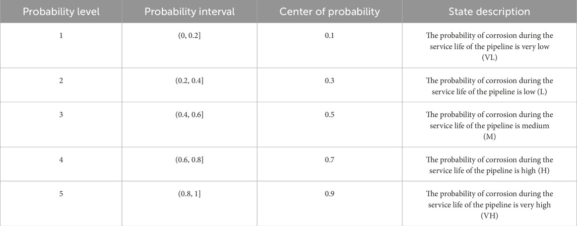
Table 2. Probability level criteria for root node occurrences.

Based on the systematic combing and analysis of historical data, this study adopts the extreme difference method to construct a five-level classification evaluation system. The full distance range of the data is determined by the extreme value method, and the research parameters are divided into five consecutive grade intervals by applying the principle of equal distance grading, and the frequency distribution statistics are performed on the number of samples in each interval, which in turn calculates their proportionate weights. The priori probabilities of some variables obtained based on historical data are shown in Table 3.

Table 3

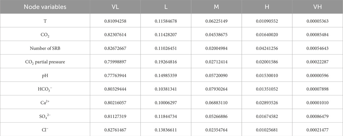
Table 3. Prior probabilities of some variables based on historical data.

In Bayesian network analysis, many factors possess uncertainty. This study primarily employs fuzzy set theory to address data uncertainty (Zou and Yue, 2020). The probabilities of input events are treated as fuzzy numbers within fuzzy set theory, with these assignments derived from expert knowledge. In practice, when prior probabilities cannot be accurately obtained from historical data, expert knowledge serves as a crucial and viable method for acquiring objective failure data of input events. During this process, fuzzy set theory is utilized to resolve the ambiguity, imprecision, and subjectivity inherent in expert knowledge (Faisal and Ebrahim, 2014).

When determining prior probabilities using expert knowledge, the concept of “fuzziness” is introduced to categorize the probability levels of root nodes. The probability level of a root node is vaguely described through the central value of a probability interval. Experts can assess the state of root nodes based on these probability levels. The weighting of experts is determined by factors such as educational background, years of experience, and level of expertise.

Due to varying educational levels and professional backgrounds, knowledge from multiple experts may be inconsistent. Therefore, it is necessary to aggregate the subjective opinions of multiple experts regarding input events into a single opinion. Various techniques are available for aggregating knowledge from different experts, among which the weighted average method is the simplest, allowing for aggregation based on the prior weights of parameters. The Equation 2 is used to aggregate the knowledge of m experts.

$P_i=\frac{{\sum }_{j=1}^m{w}_j{P}_{ij}}{{\sum }_{j=1}^m{w}_j}(2)$

where P_i represents the aggregated fuzzy number of input event i; P_ij denotes the fuzzy number of input event i provided by expert j; w_j is the weight assigned to expert j; and m stands for the number of experts.

The estimated fuzzy numbers need to be converted into crisp values (Wang et al., 2022). This study employs the max-min aggregation method to carry out the defuzzification process. The maximum fuzzy set and the minimum fuzzy set are represented as Equations 3, 4, respectively.

$f_{\max }\left(x\right)=\left\{\begin{array}{cc}x,& 0\le x\le 1\\ 0,& \text{others}\end{array}\right.(3)$

$f_{\min }\left(x\right)=\left\{\begin{array}{cc}1-x,& 0\le x\le 1\\ 0,& \text{others}\end{array}\right.(4)$

By solving the membership function, the maximum fuzzy set, and the minimum fuzzy set, the left and right scores of the fuzzy set (P) can be calculated. The fuzzy possibility score (FPS) of the fuzzy number P can be determined by Equation 5.

$FPS\left(P_i\right)=\left[FP{S}_{Right}\left(P_i\right)+1-FP{S}_{Left}\left(P_i\right)\right]/2(5)$

The FPS can be transformed into a failure probability using the Equations 6, 7.

$p_f=\left\{\begin{array}{l}\frac{1}{{10}^k}FPS\ne 0\\ 0FPS=0\end{array}\right.(6)$

$k=2.301\times {\left[\left(1-FPS\right)/FPS\right]}^{1/3}(7)$

In this study, three experts were invited to estimate the probabilities of the basic events, and their information is presented in Table 4. The analytic hierarchy process (AHP) was employed to determine the weights of their opinions (w). The expertise of the experts was assessed based on three aspects: job category, work experience, and educational level. The weights assigned to the experts were derived from the overall ranking of the hierarchical structure, as shown in Table 4.

Table 4

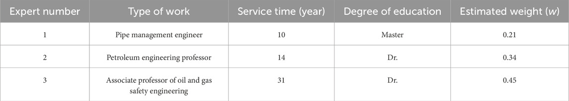
Table 4. Expert information and estimated weights.

Selected examples of the experts’ assessments regarding the input events are delineated in Table 5. To address the uncertainties inherent in subjective judgments, fuzzy numbers are utilized, and a weighted average approach is adopted to aggregate the diverse expert opinions. The integration of expert knowledge with fuzzy set theory facilitates the derivation of prior probabilities for the root nodes, as encapsulated in the aforementioned equations. Subsequently, these probabilities are instrumental in the constructed Bayesian Network, enabling the computation of probability distributions via Bayesian Network inference.

Table 5

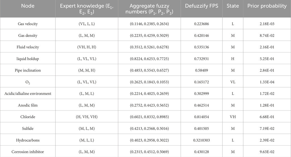
Table 5. The derivation process of selected nodes’ prior probabilities.

2.3 Prediction of internal corrosion probability in pipelines

The objective of the study is to calculate the probability of corrosion given certain causes, hence causal reasoning is employed. The results of this reasoning are illustrated in the figure below.

It should be noted that the “state” in Figure 3 correspond to the corrosion probability classes presented in Table 2. Taking “T” in Figure 3 as an example, the value of “state” corresponds to the priori probabilities of “T” in Table 3, “state 0” corresponds to the “VL” state, “state 1” corresponds to the “L” state, “state 2” corresponds to the “M” state, “state 3” corresponds to the “H” state, and “state 4” corresponds to the “VH” state.

Figure 3

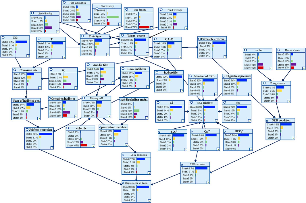
Figure 3. Causal reasoning results of Bayesian network.

2.4 Case study for model validation

This study takes the No. 1 pipeline from a shale gas field in Sichuan Province, China, as an engineering case study. A total of 147 excavation points over the past 3 years serve as the model validation samples. The state of corrosion is determined based on the wall thickness loss measured during excavation. Parameters such as pressure, temperature, average fluid velocity, liquid holdup, and others are represented by data from the pipeline inlet near the time of excavation or from separator sampling tests. Consequently, a total of 147 sets of pipeline corrosion samples were collected for the validation of the probability model. These 147 samples are listed in Supplementary Appendix Table 1. Figure 4 illustrates the discrepancy between the corrosion degrees predicted by the Bayesian network model and the measured corrosion degrees.

Figure 4

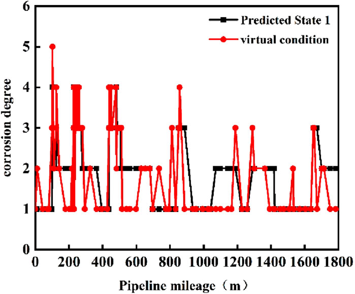
Figure 4. Comparison of predicted and measured corrosion degrees.

As depicted in Figure 4, the maximum relative error between the corrosion probability predicted by the model and the field-measured data reaches two degrees (approximately 40%). This indicates that the prediction accuracy remains relatively low. Therefore, to enhance the precision of the model, it is considered to incorporate common cause failure analysis to refine the internal corrosion probability model.

3 Modified model by considering common cause failure analysis

3.1 Overview of common cause failure

When two or more elements within a system fail simultaneously due to the same cause, it is referred to as common cause failure (Gu et al., 2018). Currently, models for analyzing common cause failures include the β factor model, α factor model, square root model, basic parameter model, and mixed parameter model, among others. The β factor model requires the determination of only one parameter and does not need to consider the issue of data loss, hence this study employs the β factor model for common cause failure analysis.

In calculations using this model, only two failure scenarios are considered: one is the independent failure of the unit itself, and the other is the simultaneous failure of all units due to a common cause. Therefore, the failure probability of a unit consists of two parts, namely, the unit’s own failure probability and the common cause failure probability, which can be calculated according to the Equation 8.

$Q=Q_1+Q_2(8)$

where Q₁ represents the failure probability of the unit itself; Q₂ denotes the common cause failure probability; and Q is the system failure probability.

The symbols λ₁, λ₂, and λ represent the failure rate of the unit itself, the common cause failure rate, and the failure rate of the entire system, respectively. The calculation expression for the common cause factor β is given by the Equation 9:

$\beta =\frac{Q_2}{Q}=\frac{Q_2}{Q_1+Q_2}=\frac{1-e^{-{\lambda }_{2}t}}{1-e^{-{\lambda }_{2}t}}=\frac{1-e^{-{\lambda }_{2}t}}{\left(1-e^{-{\lambda }_{1}t}\right)+\left(1-e^{-{\lambda }_{2}t}\right)}\approx \frac{{\lambda }_2}{\lambda }=\frac{{\lambda }_2}{{\lambda }_1+{\lambda }_2}(9)$

Generally, the β factor ranges from 0 to 0.25 (where 0 indicates no occurrence of common cause failures). Research shows that the value of the β factor accounts for 0.1%–10% of the hardware failure rate. If the related components are relatively sensitive to external conditions, they will have a higher β value. To simplify the calculation and analysis, when considering the impact of common cause failures on multi-state systems, it is assumed that the impact of common cause failures on the system is decisive, meaning that when components are affected by common cause failures, they completely fail.

Under general circumstances, if there are k components failing out of m units, the failure probability for these k components is given by the Equation 10:

$Q_k=\left\{\begin{array}{cc}\left(1-\beta \right)Q_t& \left(k=1\right)\\ 0& \left(1<k<m\right)\\ \beta Q_t& \left(k=m\right)\end{array}\right.(10)$

where Q_k represents the total failure probability of the unit; and Q_t signifies the common cause failure probability of the unit.

The β factor varies depending on the system in question. The value of the β factor also differs when the system is in different states. The estimation formula for the β factor is as Equation 11 shows:

$\widehat{\beta }=\frac{{\sum }_{k=2}^{m}k{n}_k}{{\sum }_{k=1}^{m}k{n}_k}(11)$

where n_k represents the number of common cause failure events associated with a specific component.

The β factor model solution examples are as follows:

In Figure 5, nodes X₁ and X₂ represent the independent failure factors of the components, and node C is the common cause failure factor, which can be determined through the β factor model. After adding the common cause node C, the common cause failure factor C is in series with nodes X₁ and X₂, while the intermediate nodes M₁ and M₂ remain in parallel. Each component has the potential to fail independently, or to experience multiple-component common cause failures with several components, or to have a common cause failure where n components fail simultaneously. Since the probability of multiple components failing independently at the same time is extremely low, this study does not consider it for the time being. The value of the β factor is estimated, and the common cause failure factor for components X₁ and X₂ is taken as 0.1 (Song, 2021).

Figure 5

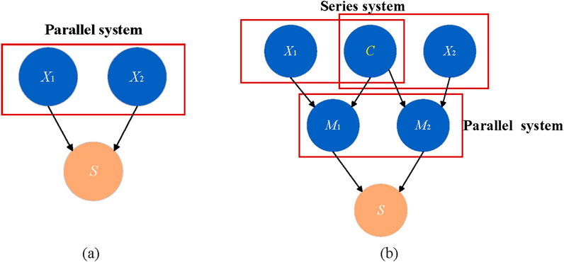
Figure 5. Bayesian network of a two-component parallel system: (a) without consideration of common-cause failures; (b) with common cause failure.

3.2 Bayesian network model considering common cause failures

The common cause failure groups are identified through common cause failure analysis. The corresponding modeling is completed using the explicit modeling method, and relevant common cause nodes are introduced into the Bayesian network model. Conditional probability tables are generated according to the logical relationships, ultimately producing a Bayesian network model that includes common cause failures. Through the analysis of the shale gas gathering pipeline structure, it is determined that gas velocity and fluid velocity, as well as pipeline inclination and liquid holdup, satisfy the conditions for common cause failures, forming common cause failure groups. The established Bayesian network model that includes common cause failures is shown in Figure 6.

Figure 6

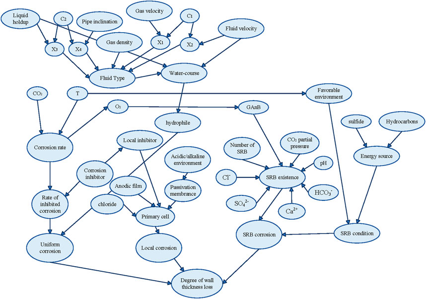
Figure 6. Bayesian network model considering common cause failures.

3.3 Updated prediction and analysis of corrosion probability

The results of the reasoning are illustrated in Figure 7. Figure 8 shows a comparison between the model’s predicted results and the actual measured results. After considering common cause failures, the maximum relative error between the corrosion levels predicted by the model and the field measurement data has been reduced to below 20%. Clearly, the probability prediction analysis becomes more accurate when common cause failures are taken into account. Therefore, it is necessary to consider common cause failures when using Bayesian networks to predict corrosion probabilities in shale gas pipelines. This method holds significant practical importance for engineering guidance.

Figure 7

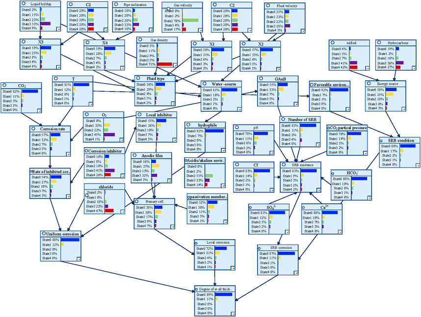
Figure 7. Causal reasoning results of Bayesian network.

Figure 8

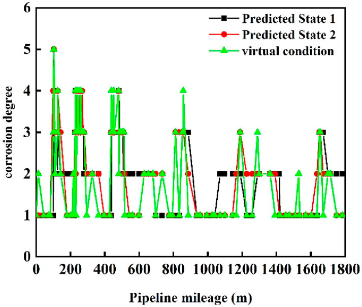
Figure 8. Comparison of predicted and measured corrosion degrees.

4 Conclusion

The following conclusions can be drawn from this study:

(1) A Bayesian network-based probabilistic model for internal corrosion of shale gas pipelines was established, and the internal corrosion probability of pipelines in a shale gas field in Sichuan Province, China, was predicted. The maximum error between the predicted results and the measured results reached 40%.

(2) Using a modified model that considers common cause failure for predicting the internal corrosion probability of pipelines, the error between the predicted results and the measured results was reduced to below 20%.

(3) Through qualitative analysis and quantitative evaluation of the Bayesian network corrosion probability model that considers common cause failure, the corrosion locations and times of pipelines can be effectively determined, providing reasonable guidance for corrosion prediction in shale gas pipelines.

(4) The established uniform corrosion failure probability model and pitting corrosion failure probability model only consider changes in one-dimensional space. Subsequent research could consider the impact of multi-dimensional space to further study the internal corrosion probability prediction technology for shale gas pipelines, making the model more mature.

Data availability statement

The original contributions presented in the study are included in the article/Supplementary Material, further inquiries can be directed to the corresponding author.

Author contributions

JG: Writing – review and editing. JS: Writing – review and editing. MW: Writing – review and editing. KY: Writing – review and editing. JZ: Writing – review and editing. YL: Writing – review and editing. XZ: Writing – original draft, Writing – review and editing.

Funding

The author(s) declare that financial support was received for the research and/or publication of this article. The APC was funded by PetroChina Southwest Oil and Gasfield Company. The funder was not involved in the study design, collection, analysis, interpretation of data, the writing of this article, or the decision to submit it for publication.

Acknowledgments

The authors thank Jing Li and Jun Shen for valuable discussion.

Conflict of interest

Authors JG, JS, MW, KY, and JZ were employed by PetroChina Southwest Oil and Gasfield Company. Author YL was employed by Sinopec Corp.

The remaining author declares that the research was conducted in the absence of any commercial or financial relationships that could be construed as a potential conflict of interest.

Generative AI statement

The author(s) declare that no Generative AI was used in the creation of this manuscript.

Publisher’s note

All claims expressed in this article are solely those of the authors and do not necessarily represent those of their affiliated organizations, or those of the publisher, the editors and the reviewers. Any product that may be evaluated in this article, or claim that may be made by its manufacturer, is not guaranteed or endorsed by the publisher.

Supplementary material

The Supplementary Material for this article can be found online at: https://www.frontiersin.org/articles/10.3389/fmats.2025.1575960/full#supplementary-material

References

Ayello, F., Jain, S., Sridhar, N., and Koch, G. (2014). Quantitive assessment of corrosion probability—a bayesian network approach. Pitting Houst. tx 70 (11), 1128–1147. doi:10.5006/1226

CrossRef Full Text | Google Scholar

Du, Y. (2019). Vulnerability assessment of the defense system and typical sites of the Ming Great Wall in Qinghai. Lanzhou University.

Google Scholar

Faisal, A., and Ebrahim, M. A. (2014). Integrating lean principles and fuzzy bow-tie analysis for risk assessment in chemical industry. J. loss Prev. process industries 29, 39–48. doi:10.1016/j.jlp.2014.01.006

CrossRef Full Text | Google Scholar

Gu, Y. C., Shen, Y. J., Zhang, Q. X., and Cai, Q. (2018). Reliability analysis of multi-state co-causal failure system based on Bayesian network. Mech. Des. Res. 34 (02), 1–4+9. doi:10.13952/j.cnki.jofmdr.2018.0045

CrossRef Full Text | Google Scholar

Han, J. Y., Dai, C. H., and Li, Y. J. (2024). Failure analysis of jet fuel storage and transportation refueling control system based on bowtie-Bayesian network. J. Civ. Aviat. 8 (05), 137–142. doi:10.3969/j.issn.2096-4994.2024.05.029

CrossRef Full Text | Google Scholar

Hu, Y., Jing, J., and Chen, M. (2023). Risk evaluation of oil and gas pipeline in high consequence area based on dynamic Bayesian network. Pet. Eng. Constr. 49 (05), 32–37. doi:10.3969/j.issn.1001-2206.2023.05.006

CrossRef Full Text | Google Scholar

Li, L., Du, N., Cui, J., Chen, K., Long, X., Zhang, Y., et al. (2020). The causes and corrosion mechanisms of internal corrosion in gathering pipelines of a production plant in Changqing Oilfield. Corros. and Prot. 41 (2). doi:10.11973/fsyfh-202002013

CrossRef Full Text | Google Scholar

Mohammed Nor, A. (2013). The effect of turbulent flow on corrosion of mild steel in high partial CO₂ environments. Ohio University.

Google Scholar

Palumbo, G., Kollbek, K., Wirecka, R., Bernasik, A., and Górny, M. (2020). Effect of CO2 partial pressure on the corrosion inhibition of N80 carbon steel by gum Arabic in a CO2-water saline environment for shale oil and gas industry. Materials 13 (19), 4245. doi:10.3390/ma13194245

PubMed Abstract | CrossRef Full Text | Google Scholar

Shabarchin, O., and Tesfamariam, S. (2016). Internal corrosion hazard assessment of oil and gas pipelines using Bayesian belief network model. J. loss Prev. process industries, 479–495. doi:10.1016/j.jlp.2016.02.001

CrossRef Full Text | Google Scholar

Shan, G., Francois, A., and Narasi, S. (2019). Application of probabilistic model in pipeline direct assessment. J. loss Prev. process industries, 459–474. doi:10.5006/1754

CrossRef Full Text | Google Scholar

Song, Y. (2021). Comprehensive reliability assessment of systems integrating multi-source uncertainties and complex failure characteristics. University of Electronic Science and Technology of China.

Google Scholar

Wang, P., Sun, Z., Zhang, F., and Xiao, G. (2022). Reliability analysis model of multi-stage task system considering probabilistic common cause failure. Syst. Eng. Electron. 44 (12), 3887–3898. doi:10.12305/j.issn.1001-506X.2022.12.35

CrossRef Full Text | Google Scholar

Xiang, W., and Zhou, W. (2020). Integrated pipeline corrosion growth modeling and reliability analysis using dynamic Bayesian network and parameter learning technique. Struct. and Infrastructure Eng. Maintenance 16, 1161–1176. doi:10.1080/15732479.2019.1692363

CrossRef Full Text | Google Scholar

Xie, M., and Zhang, Q. (2018). Research on corrosion problems in the surface gathering and transportation system of Changning shale gas field. Pipeline Prot. 4. doi:10.26914/c.cnkihy.2018.002617

CrossRef Full Text | Google Scholar

Yue, M., and Wang, Y. (2018). Causes of corrosion and protective measures for downhole tubing and surface gathering pipelines in shale gas wells. Drill. and Prod. Technol. 5 (41). doi:10.3969/J.ISSN.1006-768X.2018.05.38

CrossRef Full Text | Google Scholar

Zou, C., and Yue, S. (2020). Bayes probability correction method for knowledge element events based on DS and fuzzy set theory. Statistics Decis. 4 (9), 30–35. doi:10.13546/j.cnki.tjyjc.2020.09.006

CrossRef Full Text | Google Scholar