 Jouni Suhonen
 Joel Kostensalo
- Department of Physics, University of Jyvaskyla, Jyväskylä, Finland
Quenching of the weak axial strength gA is discussed and relations of this quenching to the nuclear matrix elements of double beta decays are highlighted. An analysis of Gamow-Teller transitions in the mass range A = 62 − 142 is presented and its results are compared with those of many previous works. The enhancement of the axial charge is discussed for first-forbidden pseudoscalar β transitions. Higher-forbidden β transitions are introduced and their role in determining the effective value of gA is examined, in particular from the point of view of the β-decay half-lives and the shapes of electron spectra of forbidden non-unique β transitions.
1. Introduction
Double β decay (ββ decay) has been under intensive discussion for the last decades from the point of view of both nuclear theory and ββ-decay experiments. The interesting decay mode is the neutrinoless ββ (0νββ) decay which is mediated, e.g., by a massive Majorana neutrino, which is exchanged between the two decaying nucleons. Thus the 0νββ decay implies also the breaking of lepton-number conservation. The high stakes involved in the detection of 0νββ decay have made the associated theoretical and experimental aspects highly important, in particular the calculation of the involved nuclear matrix elements (NMEs). The NMEs of 0νββ decays have been computed for decades using a number of different nuclear-structure approaches (for older calculations see the review [1] and for the more recent ones see [2, 3]). Most of these calculations have been done by using the framework of the QRPA (quasiparticle random-phase approximation [4]). Also many calculations have been performed using the interacting shell model (ISM, see e.g., [5–7]) and the microscopic interacting boson model (IBM-2, see e.g., [8]).
Besides the problems with the calculations of the NMEs of 0νββ decay there is an other severe problem, namely the one related to the value of the weak axial coupling gA. For low-energy processes, like the β decay or the two-neutrino ββ (2νββ) decay [1], the nucleonic charged weak current is simply
where Ni (Nf) is the initial-state (final-state) nucleon spinor and γs are the usual Dirac matrices. Here gV = 1.0 is the weak vector coupling and its value is protected by the CVC (Conserved Vector Current) hypothesis [9]. The value gA = 1.27 of the weak axial coupling has been obtained from the decay of free neutron [10], Ni = n in (1), into free proton, Nf = p in (1). For the 0νββ decay the values of these weak couplings are altered by the high energy scale (q ~ 100 MeV) of the exchanged momentum q between the decaying nucleons and the Majorana neutrino. In addition, induced currents become involved in the decay (see e.g., [11]). The evolution of the value of gA with the magnitude of the exchanged momentum q has been discussed in Menéndez et al. [12] and an extensive discussion of the effective value of gA has been carried out in the review [13].
For the two-neutrino ββ decay from the initial 0+ state () to the final 0+ state () the decay rate is directly proportional to the fourth power of gA as given by
where Δ is the nuclear mass difference between the initial and final 0+ ground states, Mi is the mass of the initial nucleus, me the electron rest mass and is the absolute energy of the nth 1+ state. Furthermore, is the left-branch NME and the right-branch NME for the nth 1+ state, as shown schematically in Figure 1. The NMEs and are the usual Gamow-Teller NMEs. In this case the low-momentum form (1) of the nucleon current is applicable and the quenching of gA can be studied through allowed Gamow-Teller β decays of low-energy nuclear states, as described in section 3 of this article.
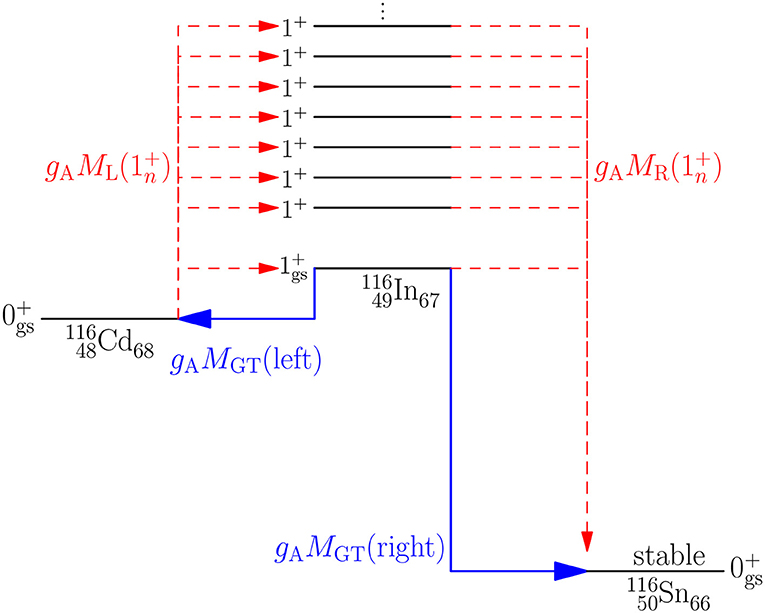
Figure 1. Schematic representation of the β and 2νββ transitions in the mass A = 116 triplet. Shown are the 0+ ground state of the initial nucleus 116Cd, the 0+ ground state of the final nucleus 116Sn and the 1+ states of the intermediate nucleus 116In of the 2νββ decay. Also the left-branch and right-branch NMEs for both decay modes are presented.
For the 0νββ decay from the initial 0+ state () to the final 0+ state () the decay rate is given by
where the Fermi NME is proportional to and the Gamow-Teller and tensor NMEs, and , are proportional to . The Gamow-Teller NME is the leading one and has the constitution
where the sum is over all multipole states Jπ in the intermediate nucleus and the effective axial couplings for 0νββ decay, , are, in principle, multipole dependent. All the details of the 0νββ-decay transitions are included in the operator . The low-q limit of these couplings is
where q is the exchanged momentum. For the Jπ = 1+ multipole this low-q limit is the “usual” axial coupling
relevant for the Gamow-Teller and 2νββ decays. For the sake of simplicity, the notation gA will be used also for the other multipoles . The gA for higher multipoles can be studied through half-lives and electron spectral shapes of forbidden β decays, as discussed in section 4 of this article.
2. Nuclear Models
In this section we briefly describe the many-body aspects of the nuclear models which are mentioned later in this article. These models have been used to study the β-decay and ββ-decay NMEs and the associated effective values of the axial coupling. It should be noted here that these are not the only models that can (potentially) describe these features. These other nuclear models can be based on modern energy-density functionals or thermofield-dynamics formalism, as also on Monte-Carlo shell model, etc. A comprehensive list of these nuclear models and the associated references are given in section 5.4. of the very recent review article [14].
• ISM: The ISM (interacting shell model) is a many-body framework that uses a limited single-particle valence space, typically one harmonic-oscillator major shell or one nuclear major shell. In the ISM one forms all the possible many-nucleon configurations in a given single-particle valence space, each configuration described by one Slater determinant, and diagonalizes the nuclear (residual) Hamiltonian in the basis formed by these Slater determinants. In this way the many-body features are taken into account exactly but only in a restricted valence space, typically leaving out one or two spin-orbit-partner orbitals from the model space.
• Spherical pnQRPA: The proton-neutron version of the QRPA (pnQRPA) uses two-quasiparticle excitations that are built from a proton and a neutron quasiparticle. Here only the spherical pnQRPA, based on a spherical nuclear mean field, is described. The pnQRPA model framework enables description of odd-odd nuclei starting from an even-even reference nucleus where the quasiparticles are created, e.g., through the BCS (Bardeen-Cooper-Schrieffer) procedure [15]. The advantage of the pnQRPA theory is that it can include large single-particle valence spaces in the calculations and there arise no problems associated with spin-orbit-partner orbitals since they can easily be accommodated in the valence space. On the other hand, the pnQRPA has a limited configuration space. Schematic or G-matrix-based boson-exchange Hamiltonians have widely been used in the pnQRPA calculations. A frequently used extension of the pnQRPA framework is the renormalized QRPA (RQRPA) [16, 17]. One particular problem with the pnQRPA calculations is the determination of the value of the particle-particle interaction parameter gpp, used to scale the particle-particle part of the proton-neutron two-body interaction matrix elements [18, 19]. Usually the value of this parameter has been determined by using β-decay or 2νββ-decay data. The particle-hole parameter, gph, of the proton-neutron two-body interaction is usually determined by adjusting the parameter such that the phenomenological or experimental energy of the Gamow-Teller giant resonance is reproduced [20, 21]. The spherical pnQRPA has been applied to the description of ββ decays (see e.g., [22–25]) and it has also been used in β-decay studies (see e.g., [26–28]).
• MQPM: The microscopic quasiparticle-phonon model (MQPM) describes states of odd-A nuclei starting from the adjacent even-even reference nuclei. The MQPM states are generated by combining proton or neutron one-quasiparticle excitations of the reference nucleus with three-quasiparticle excitations built by coupling a proton or neutron quasiparticle to a QRPA phonon. A QRPA phonon is a proton-proton-plus-neutron-neutron excitation of an even-even reference nucleus. The MQPM creation operator creates a state |kjm〉 in an odd-A nucleus by the action
with the excitation operator given by
where is a QRPA phonon creation operator [15] and the a† operators create BCS quasiparticles. Since the MQPM states (8) contain the three-quasiparticle components special care should be taken when solving the MQPM equations of motion for the amplitudes and in order to handle the over-completeness and non-orthogonality of the quasiparticle-phonon basis. For details see Toivanen and Suhonen [29, 30].
• IBM-2: The interacting boson model (IBM) is a theory framework based on s and d bosons which have as their microscopic paradigms the 0+ and 2+ angular-momentum-coupled collective fermion pairs present in nuclei. An extension of the IBM is the microscopic IBM (IBM-2) where the proton and neutron degrees of freedom are explicit. The IBM-2 is a sort of phenomenological version of the ISM, containing the seniority aspect and the restriction to one magic shell in terms of the single-particle valence space. The Hamiltonian and the transition operators are constructed from the s and d bosons as lowest-order boson expansions with coupling coefficients to be determined by fits to experimental data on low-lying energy levels and E2 γ transitions. However, the fitting does not use the spin or isovector data available from β decays. The extension to the microscopic interacting boson-fermion model (IBFM-2) [31] enables the description of odd-A nuclei. Here problems arise from the interactions between the bosons and the extra fermion in the Hamiltonian, and from the transition operators containing a host of phenomenological parameters to be determined in some meaningful way.
3. Quenching of GA in Gamow-Teller β Decays
The half-life of allowed Gamow-Teller β decays can be written as
where is the integrated shape function and the constant κ has the value [32]
θC being the Cabibbo angle. In order to simplify the formalism it is usual to introduce unitless kinematic quantities , , and , where We is the total energy of the emitted charged lepton (electron or positron), pe is the electron/positron momentum and W0 is the end-point energy, i.e., the total energy of the emitted leptons, and hence the maximum energy of the emitted electron/positron. With the unitless quantities the integrated shape function can be expressed as
where F0(Zf, we) is the Fermi function taking into account the interaction of the final-state charged lepton with the positive charge of the final nucleus (with charge number Zf). The integration is performed over the total scaled energy of the emitted electron/positron.
The shape factor C(we) of Equation (11) can be expressed for the pure1 Gamow-Teller Ji → Jf = Ji ± 1 transitions as
where MGT is the Gamow-Teller NME (assumed to be real, as usual) and Ji (Jf) the angular momentum of the initial (final) state. Here the axial coupling gA is the low-q limit (6). Since the shape factor (12) does not depend on the lepton variables it can be taken out of the shape function (11) and the rest constitutes the universal phase-space factor
usually quoted for the allowed (Fermi and Gamow-Teller) β decays. At this point it should be noted that a new method of calculation of these phase-space factors was introduced in Stoica et al. [33]. These phase-space results contribute to calculations of β-decay rates for nuclei far away from the stability line. Using the phase-space factor f0, the half-life (9) can be expressed in a more familiar form using the reduced transition probability BGT:
What is usually quoted in literature are the log ft values
which are 10-base logarithms of the product of the half-life and the universal phase-space factor.
By using Equations (14) and (15) one can extract from the experimental log ft value the magnitude of the experimental Gamow-Teller NME in the form |gAMGT|. Here one has to note that only the product of the NME and the weak axial coupling gA can be extracted. These products can be extracted from both the left-branch, |gAMGT(left)|, and right-branch, |gAMGT(right)|, β decays as shown schematically in Figure 1. These extracted products are shown in Tables 1, 2 for the left (third column) and right (fifth column) transitions from/to the central nucleus of the triplet of nuclei of column two. A sample of these triplets are shown in Figure 2. There four mass triplets A = 110, 116, 128, 136 are displayed with a central nucleus feeding the lateral ones, thus constituting the left-branch and right-branch of β transitions. These triplets host also double beta decays, with β−β− decays for the masses A = 110, 116, 128 and double electron-capture (EC) decay for A = 136. For the double EC decay the log ft of the right-branch decay is not known and thus this triplet is omitted from the subsequent decay analysis whereas all the other triplets are included. In the figure it is also shown that there is no available data on the decays of the low-lying 2− states in these triplets. These decays are relevant for the first-forbidden unique β transitions of section 4.2, mediated by a rank-2 tensor. They are also quite important for the neutrinoless ββ-decay NMEs.
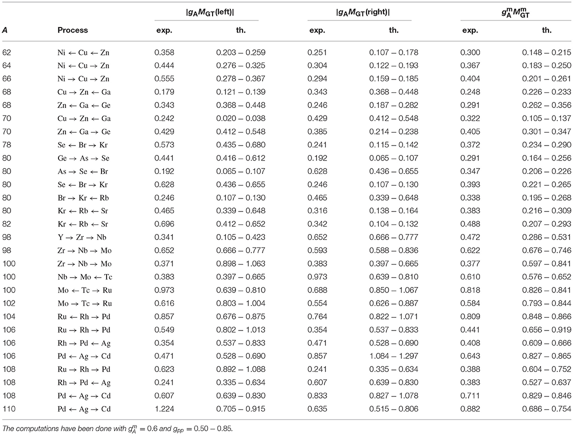
Table 1. Experimental and computed geometric means of the NMEs for A = 62 − 110.
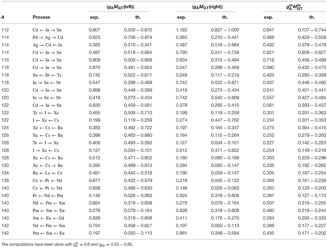
Table 2. Experimental and computed geometric means of the NMEs for A = 112 − 142.
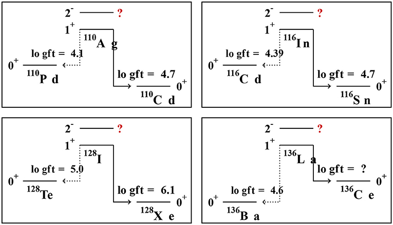
Figure 2. Experimental log ft values of the left-branch and right-branch β transitions in four triplets of nuclei. It is also shown that no data on the decays of the 2− states are available in these triplets.
As can be seen in Tables 1, 2, the extracted experimental left-branch and right-branch NMEs differ sometimes considerably from each other and these differences are rather erratic. In order to stabilize this behavior one may use the geometric mean of the left and right NMEs:
where the geometric mean of both the left-branch and right-branch NMEs and axial couplings has been computed. The corresponding experimental NMEs are shown in column seven in Tables 1, 2. These NMEs do not behave quite as wildly as the individual left-branch and right-branch NMEs.
The experimental left-branch, right-branch and mean NMEs can be compared with the corresponding computed NMEs listed in columns four, six and eight in Tables 1, 2. The computed NMEs are obtained by using the pnQRPA (see section 2) in the following single-particle model spaces:
These single-particle valence spaces have been chosen such that they are expected to capture the relevant features of the low-lying states in the triplets of nuclei, such that the involved left-branch and right-branch β transitions are described as well as possible within the framework of the pnQRPA model. In the course of the calculations the pairing parameters were fitted to reproduce the experimental pairing gaps extracted from the available data [34] on nucleon separation energies. The particle-hole parameter gph was fitted to reproduce the empirical location of the giant Gamow-Teller resonance (see [35] for fitting also to more general spin-multipole resonances).
The particle-particle parameter gpp and the strength of the axial coupling were left as free parameters in the calculations. According to the Gamow-Teller β-decay study [36], performed for a number of nuclei in the mass range A = 100 − 136, a good overall value for the particle-particle parameter is gpp ≈ 0.7. In the present study we vary the values of this parameter in the range gpp = 0.50 − 0.85 to have a feeling of the effects of the variation of gpp on the values of the computed NMEs. This variation is shown in Tables 1, 2, in columns four and six for the left-branch and right-branch NMEs, and in the last column for the mean NMEs (16). The variations in the values of the individual NMEs are usually (much) larger than in the values of the mean NMEs, thus justifying the use of the geometric mean of the left-branch and right-branch NMEs, instead of the individual NMEs. For the mean strength of the axial coupling we have taken the constant overall value which was found to be a good average value in the study [36] for the A = 100 − 136 mass range. Our adopted values of gpp = 0.67 (plus the variation in gpp described above) and gA = 0.6 are also in good agreement with the average values of these parameters deduced from the extensive analyses of the Gamow-Teller β decays conducted in the study [37].
A further comparison of the calculated and experimental Gamow-Teller NMEs has been conducted in Figures 3–6. In these figures the computed values of the mean NMEs (16) are presented for gpp = 0.67 (solid line with open circles) and the hatched area represents the variations in these values induced by the adopted range gpp = 0.50 − 0.85 of variations in the value of the particle-particle interaction parameter. The extracted experimental NMEs are represented by a dashed line with filled circles.
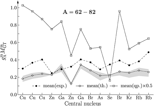
Figure 3. Mean experimental and theoretical NMEs (Table 1, last two columns) for the mass range A = 62 − 82. The hatched area describes the uncertainty of the calculations (the range gpp = 0.50 − 0.85 in Table 1). Also the NMEs in the two-quasiparticle approximation have been plotted for comparison (note the scaling of these NMEs by a factor one-half in order to save vertical space in the figure).
From Figures 3–6 one notices that in the mass range A = 62 − 82 (Figure 3) the magnitude of the computed mean NME is almost everywhere slightly below that of the experimental one whereas in the mass region A = 98 − 110 (Figure 4) the magnitude of the computed mean NME is above that of the experimental mean NME. In both mass regions the staggering of the computed and experimental mean NMEs is similar. In the mass range A = 112 − 124 (Figure 5) the experimental mean NME is mostly larger than the computed one but the staggering of both are quite similar. For the heaviest triplets, A = 126 − 142 (Figure 6), the values of the experimental mean NMEs are larger than those of the computed ones, the difference increasing with increasing mass. Still, in the staggering similarities between the two NMEs are to be seen.
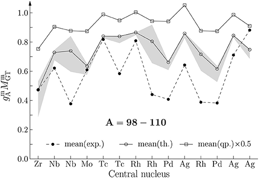
Figure 4. The same as in Figure 3 for the mass range A = 98 − 110.
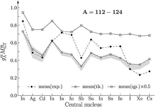
Figure 5. The same as in Figure 3 for the mass range A = 112 − 124, with the mean NMEs corresponding to Table 2.
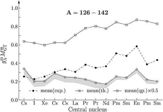
Figure 6. The same as in Figure 5 for the mass range A = 126 − 142.
In Figures 3–6 also the magnitudes of the proton-neutron two-quasiparticle NMEs are presented (solid line with open squares) for comparison. The corresponding spin-orbit-partner configurations give the strongest contributions to the mean NMEs and these configurations are
Here it should be noted that these configurations are not the same as the leading contributions quoted in the study [38] since there the two-quasiparticle configurations closest to the respective Fermi surfaces were taken. The magnitudes of the two-quasiparticle mean NMEs are far too large implying a strong quenching of the mean NME when going from the simple two-quasiparticle approximation to the more sophisticated pnQRPA model. This large reduction can be associated with spin-isospin correlations missing in the two-quasiparticle approximation but taken into account in the pnQRPA framework, as discussed extensively in Ejiri and Suhonen [38]. In the two-quasiparticle NMEs there are also some staggering in the magnitude, but usually (much) less than in the pnQRPA and experimental NMEs. Sometimes this staggering is out of phase with the pnQRPA staggering (and the experimental one) indicating that the spin-isospin correlations are crucial in order to reproduce the trends of the experimental mean NMEs.
The error bars of the magnitudes of the computed NMEs, caused by the variation gpp = 0.50 − 0.85, are shown as hatched areas in Figures 3–6. In general, the relative variation is rather modest, in particular in the mass range A = 112 − 124 (Figure 5). The largest absolute variations are seen around the masses A = 100, A = 106 and A = 108. Generally, the upper limit of the hatched area is close to the best NME value (solid line with open circles) since this maximum NME is obtained for the lowest value gpp = 0.50 and for this value of gpp the NME is already saturated close to its maximum value at gpp = 0.0.
To give yet an other view to the comparison of the experimental and computed NMEs, one can calculate the mean value and the RMS (Root-Mean-Square) deviation of the NMEs in the four mass ranges of Figures 3–6. The result is
These ranges have been shown in Figure 7 for easy comparison. The figure shows clearly that the computed mean NMEs are smaller than the experimental ones for small (A = 62 − 82) and large (A = 126 − 142) mass numbers, whereas for the intermediate masses (A = 98 − 124) they largely overlap with the experimental ones. This means that with an overall constant one cannot reproduce the values of the experimental mean NMEs.
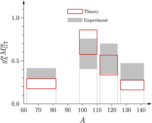
Figure 7. Ranges of the experimental and theoretical mean NMEs for different mass ranges as deduced from (19).
If one would like to match the experimental and computed average in the different mass ranges one would need a different effective value of the weak axial coupling in each of them. Matching the computed NMEs with the data leads to the following effective values
One can compare these values of effective gA ( in Figure 8) with other recent calculations in different theory frameworks. This has been done in Figure 8. In the figure the present pnQRPA results are displayed by blue horizontal solid lines. These are contrasted against the ISM-computed (for the ISM, see section 2) results of Martínez-Pinedo et al. (ISM calculations of rates of β decays [42], gray rectangle marked M-P1996 in the figure), Siiskonen et al. (ISM calculations of muon-capture transitions of different exchanged momenta with effective transition operators [44], circles with cross inside in the figure), Caurier et al. (based mainly on analyses of 2νββ decays [5], solid red horizontal lines), Horoi et al. (based mainly on analyses of 2νββ decays in the A = 124 − 136 region [6], horizontal dashed line in the figure), Kumar et al. (systematic examination of β decays with the ISM [43], dark rectangles in the A = 52 − 80 regions in the figure), Iwata et al. (ISM analysis of the ββ decays of 48Ca [7], cross at A = 48 in the figure). The studies of Faessler et al. [40] and Suhonen and Civitarese [41], marked by vertical black and green line segments, respectively, are pnQRPA studies of nuclei (100Mo, 116Cd, and 128Te) with available data on the rates of both β and 2νββ decays The analyses were performed in the aim of constraining the values of both gA and gpp simultaneously. The solid line with the zig-zag behavior is the result of the pnQRPA analysis of Suhonen [39] in the aim to constrain the possible values of gA and 0νββ NMEs in order to have a feeling of their effects on the sensitivity of the present and future 0νββ experiments.
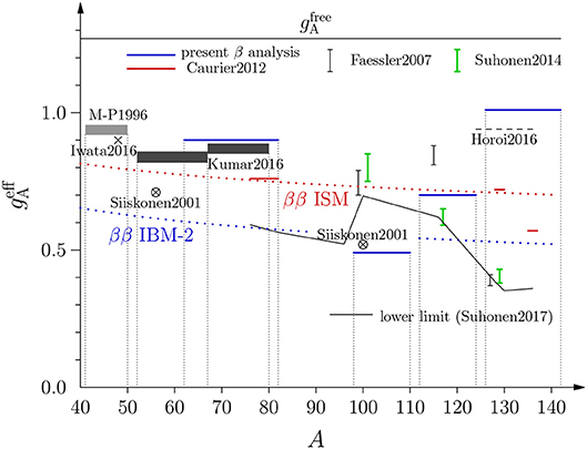
Figure 8. Effective values of gA in different theoretical β and 2νββ analyses for the nuclear mass range A = 41 − 142. The quoted references of 2νββ studies are Suhonen2017 [39], Caurier2012 [5], Faessler2007 [40], Suhonen2014 [41] and Horoi2016 [6]. These studies are contrasted with the ISM β-decay studies of M-P1996 [42], Iwata2016 [7], Kumar2016 [43] and Siiskonen2001 [44]. The red and blue dotted lines show the results of the analysis in Barea et al. [8] and quoted in Equation (21).
The red (ββ ISM) and blue (ββ IBM-2) dotted lines show the results of the 2νββ analyses of Barea et al. [8] yielding the fits
where A is the mass number and IBM-2 stands for the microscopic interacting boson model (see section 2). The IBM-2 results have been obtained by using the closure approximation for the analyzed 2νββ transitions since there are no spin-isospin degrees of freedom in IBM-2 and thus the intermediate nuclei of 2νββ decays cannot be reached.
Interesting conclusions can be drawn from the calculations shown in Figure 8. For the mass range A = 41 − 82 the present result for the effective value of gA is in striking agreement with the many shell-model calculations in the region, consistently producing the value . The same can be said about the mass regions A = 112 − 124 and A = 126 − 142 where the ISM results of Barea et al. [8] and Horoi and Neacsu [6] are quite close to the present effective values and . In the A = 126 − 142 region the ISM analyses of Caurier et al. [5] and the IBM-2 analyses of Barea et al. [8] produce smaller values of and there is a strong tension between the different ISM analyses. The present results are in line with the pnQRPA results of Suhonen and Civitarese [41] and Faessler et al. [40] for 116Cd but far off from the results of these studies for 128Te. It seems that the fit to the average value of the mean experimental β-decay NMEs brings the results of the pnQRPA analysis closer to those of the ISM, in particular for the heavy end of the presently discussed nuclei. The mass range A = 98 − 110 is the most interesting: Here a very small value is required both by the present study and the ISM study of Siiskonen et al. [44]. Also the IBM-2 result of Barea et al. [8] is consistent with these results whereas the interpolated ISM result of Barea et al. [8] and the results of Suhonen and Civitarese [41] and Faessler et al. [40] for 100Mo are in the range .
4. Quenching of GA in Forbidden β Decays
In forbidden β transitions the low-q limit (5) can be studied for different multipoles Jπ. In this section we denote all these weak axial couplings as gA for simplicity.
4.1. Theoretical Background
4.1.1. Forbidden Non-unique β Decays
The half-life of a forbidden non-unique β decay can be written in the same way as that of the allowed β decay in (9). The corresponding integrated shape function can be expressed as written in Equation (11) but the shape factor C(we) of Equation (12) has to be replaced by a much more complicated expression:
where the notation of unitless leptonic quantities was discussed in the context of Equation (11). The factor λke contains the generalized Fermi function Fke−1 [45] as the ratio
Zf being the charge number of the final nucleus. The indices ke and kν (ke, kν = 1,2,3…) are related to the partial-wave expansion of the electron (e) and neutrino (ν) wave functions, K is the order of forbiddenness of the transition, and , α ≈ 1/137 being the fine-structure constant. The nuclear-physics information is carried by the quantities MK(ke, kν) and mK(ke, kν), which are conglomerations of different NMEs and leptonic phase-space factors. For more information on the integrated shape function, see Behrens and Bühring [45] and Mustonen et al. [46].
The shape factor C(we) can be decomposed into vector, axial-vector, and mixed vector-axial-vector parts. In this decomposition the shape factor is
where the quantities CA, CV and CVA are complicated expressions including Coulomb functions, nuclear matrix elements, etc. This is the decomposition used in Haaranen et al. [47, 48] and Kostensalo et al. [49] and it enables studies of the effects caused by the ratio gV/gA on the shape factor. Integrating Equation (24) over the electron kinetic energy, we get an analogous expression for the integrated shape function (11)
where the factors , and in Equation (25) do not depend on the electron kinetic energy.
4.1.2. First-Forbidden Non-unique β Decays
For the first-forbidden non-unique β decays the shape factor (22) has to be supplemented with a ΔJ = |Ji − Jf| = 0 term [26, 45, 50, 51], where Ji (Jf) is the initial-state (final-state) spin of the mother (daughter) nucleus. In the papers (see [52–54]) the shape factor for first forbidden decays has been given in the form
where k, ka, kb, and kc contain the Coulomb functions, nuclear matrix elements and weak coupling constants. Writing the shape factor in this form is often useful for comparing the theoretical and experimental shape factors. It should be noted that the shape factors of Equations (24) and (26) are different but equivalent ways of expressing the shape factor but in the first one the terms with the same product of weak coupling constants have been collected, while in the latter the terms with the same power of electron kinetic energy we are combined.
4.1.3. Forbidden Unique β Decays
An important special case of forbidden β decays are the forbidden unique decays for which the theory simplifies considerably. The classification of forbidden unique decays by change in parity and angular momentum is presented in Table 3. For the non-unique case these are presented in Table 4.

Table 3. The change in angular momentum and parity in a Kth forbidden unique β decay.
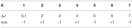
Table 4. The change in angular momentum and parity in a Kth forbidden non-unique β decay.
For unique β-decay transitions the half-life (9) can be expressed analogously to (14), valid for the Gamow-Teller β transitions. Thus we have
where fKu is the phase-space factor and gAMKu is the nuclear matrix element. The phase-space factor fKu for the Kth forbidden unique β± decay can be written as
and the corresponding shape factor can be written as (see e.g., [15, 55])
The notation was explained in the context of the allowed and forbidden non-unique β transitions, around Equations (11) and (22) and the ratio λke was given in Equation (23).
The NME in (27) can be expressed as
where the factors MKu(ab) are the single-particle matrix elements and the quantities are the one-body transition densities with ψi being the initial-state wave function and ψf the final-state wave function. The operator is a creation operator for a nucleon in the orbital a and the operator is the corresponding annihilation operator. The single-particle matrix elements are given (in the Biedenharn-Rose phase convention [15]) by
where YK is a spherical harmonic of rank K, r the radial coordinate, and a and b stand for the single-particle orbital quantum numbers. The NME is given explicitly in Suhonen [15].
4.2. First-Forbidden β Decays
The shape factor C(we) of Equation (22) contains complicated combinations of both (universal) kinematic factors and nuclear form factors [26–28]. The nuclear form factors can be related to the corresponding NMEs using the impulse approximation [45]. For the first-forbidden non-unique decays the relevant NMEs are those of the transition operators denoted here by [rank-0 tensors], [rank-1 tensors] and [rank-2 tensors]. The operators mediate pseudoscalar transitions, pseudovector transitions and pseudotensor transitions. In the non-relativistic reduction there are six matrix elements corresponding to the operators
where r is the coordinate vector and pe (qν) is the electron (neutrino) momentum, and the square brackets in the operator denote angular-momentum coupling. The nuclear matrix elements related to the first forbidden decays are suppressed relative to the Gamow-Teller matrix elements by the small momenta of the leptons, the large nucleon mass, and the small value of the fine-structure constant α.
The quenching of the effective value of gA in first-forbidden decays in the lead region was observed in the late 1960's in a study by Bohr and Mottelson [56]. In this study the so-called ξ approximation, discussed in Behrens and Bühring [45], Schopper [50], and Bohr and Mottelson [56], was adopted. The wave functions were assumed to be dominated by certain single-particle configurations around the double-magic 208Pb nucleus. For the decays mediated by the rank-1 operators in Equation (33), the obtained effective values of the weak coupling constants were
The effective value of the vector coupling constant deviates significantly from the canonical value gV = 1, pointing to large nuclear-model-dependent effects. Also the value of the axial coupling is quite low.
Next we discuss more recent and complete studies of the quenching or enhancement of the weak couplings in the first-forbidden β transitions.
4.2.1. Rank-0 Tensors
The mesonic enhancement of the γ5 NME (σ · pe of Equation (32) in the non-relativistic limit) was discussed in Kubodera et al. [57] for the pseudoscalar 0+ ↔ 0− β transitions. The enhancement of the γ5 NME stems from the renormalization of the pion-decay constant and the nucleon mass MN in nuclear medium [58] and exchange of heavy mesons [59, 60]. The γ5 NME is accompanied by a pseudo-scalar axial coupling gA(γ5). The effective value of this coupling can be expressed in terms of an enhancement factor ϵMEC through the relation
where gA is the usual axial-vector coupling strength. Related to this, a fundamental enhancement factor ϵMEC = 1.4 − 1.7, insensitive to nuclear-structure aspects, was predicted [61, 62]. In the paper of Kirchbach and Reinhardt [63] enhancements of 40 − 50% were predicted for singe-particle transitions between s1/2 and p1/2 orbitals. This work was extended by Towner [60] to include several single-particle transitions in multiple mass regions from light nuclei to A ≈ 208. Enhancement factors
were obtained.
The mesonic enhancement was considered also in the framework of the interacting shell model for A = 11 − 16. In the studies Millener and Alburger [64] and Warburton et al. [65] some 40 − 50% enhancement of the axial charge was found. Further systematic studies in the A = 11 − 16 [66] and A = 205 − 212 [53, 67, 68] regions reported mesonic enhancement factors of
Interestingly, in the lead-region practically no quenching of the σ · r operator was found with , as reported in Warburton [53, 67, 68]. The value of ϵMEC in the lead region was derived by Kubodera and Rho [58] by adopting an effective Lagrangian incorporating approximate chiral and scale invariance of QCD. The result of Kubodera and Rho was
which agrees well with the phenomenological shell-model result (39). In addition, separate studies for 50K [69] and 96Y [70] yielded enhancement factors 1.52±0.07 and 1.75±0.30. However, in the case of 50K there was no estimate of the theoretical error so the reported uncertainty is purely experimental.
Mesonic enhancement of the axial-charge matrix element, as well as the quenching of gA, was systematically studied in the previously less studied A ≈ 95 and A ≈ 135 regions by the present authors [71]. In this systematic shell-model study of the two regions, using state-of-the-art two-body interactions, a single effective value of for all axial-vector operators was used. The mesonic enhancement was found to depend on the chosen effective value of gA. Since the mesonic enhancement has been found to vary between 40 % and 100 %, the effective value of gA was extracted for several different values of ϵMEC. In the A = 92 − 97 region the results were
In the A = 133 − 139 region the results were quite similar:
This is quite strong evidence of the quenching of gA in first-forbidden decays, since significant quenching is found regardless of the exact strength of the mesonic enhancement. In Kubodera and Rho [58] it was pointed out that the mesonic enhancement should be larger for heavier nuclei, which is in line with the earlier shell-model results [53, 67, 68]. In Kostensalo and Suhonen [71] this was used to extract the effective value of gA by fitting all the available data from the previous studies. The fit of this study is shown in Figure 9. As can be seen from the figure, a suitably increasing mesonic enhancement as a function of A is seen only when gA ≈ 0.70. The linear fit obtained for the whole mass region A = 11 − 212 reads
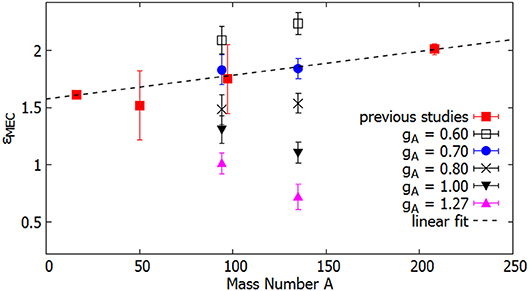
Figure 9. Mesonic enhancement factors ϵMEC of the previous studies and the study of Kostensalo and Suhonen [71] as a function of the mass number A. The red squares represent the previous systematic studies done in the A ≈ 16 and A ≈ 208 regions and the separate studies done for 50K and 96Y. The other points represent the results of Kostensalo and Suhonen [71] for different effective values of gA. The linear fit is an error-weighted fit, where the results of the previous studies and the study [71] with gA = 0.70 are used.
4.2.2. Rank-1 Tensors
Since the early findings (35) and (36) of Bohr and Mottelson [56], the effective values of the weak coupling constants related to rank-1 operators in (33) have been studied also separately using the available data on the corresponding pseudovector transitions. In Warburton [53, 67] the effective values
were obtained in the lead region, where the heavy quenching was attributed to core-polarization effects. The shell model study of Rydström et al. [72] of the transition yielded similar results:
In the work Zhi [52] half-lives of a number of nuclei at the magic neutron numbers N = 50, 82, 126 were analyzed by comparing the results of large-scale shell-model calculations with experimental data. Both Gamow-Teller and first-forbidden β decays were included in the analysis. By performing a least-squares fit to the experimental data the following quenched weak couplings were extracted
For the rank-1 operators the obtained effective value on gV is quite far from the CVC value gV = 1.0 [9]. In the recent work of Hayen et al. [73] the first-forbidden decays related to the cumulative reactor antineutrino spectrum were studied in the ISM. In this short letter type article it was not possible to give the details related to the calculations, so they are presented here for the first time. In the A = 86 − 97 region the interaction glepn [70] was used and in the region A = 133 − 142 the (unpublished) interaction jj56pnb of Alex Brown was used. For the decays with ΔJ = 1 the half-lives could not be reproduced with any reasonable gA, with the exception of the decay for which gA = 0.34(12) works, if the CVC hypothesis gV = 1 was not broken. Since there were so few decays calculated in different model spaces, it was not meaningful to start fitting the values of both gA and gV to this data. However, this might be an interesting research topic in the future. Since the previous studies, discussed above, point to gA ≈ gV, we set the two coupling constants to be equal and then fitted this value to the experimental data. As can be seen from Table 5 the recent calculations seem to also point to heavy quenching gA = gV ≈ 0.5 for the first-forbidden rank-1-tensor-mediated β decays in medium-heavy nuclei.
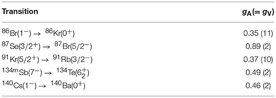
Table 5. Values of the weak couplings gA = gV needed to reproduce the experimental half-lives of the listed β transitions, mediated by rank-1 tensors (33) of the first-forbidden β decay.
4.2.3. Rank-2 Tensor
The quenching of gA related to the pseudotensor transitions mediated by the rank-2 operator (34) is best studied in the context of first-forbidden unique ground-state-to-ground-state decays in even-A nuclei, as this is the only operator at work in the leading order. In the early work [74] a systematic schematic analysis of the first-forbidden unique β decays was performed from the point of view of suppression factors stemming from the effect of E1 (electric dipole) giant resonance in the final odd-odd nucleus. In Towner et al. [75] the suppression mechanism of the first-forbidden and third-forbidden β decays of light nuclei (A ≤ 50) was studied by using simple shell-model estimates and first-order perturbation theory. The hindrance was traced to the repulsive T = 1 (isospin 1) particle-hole force.
In the work Ejiri et al. [76] 19 first-forbidden unique ground-state-to-ground-state β-decay transitions were studied. The interesting transitions are the ones where a central nucleus (here only 84Kr) is fed by a left-branch and a right-branch 2− → 0+ transition or a central nucleus (74As, 86Rb, 122Sb and 126I) is feeding the neighboring even-even nuclei by left-branch and right-branch 2− → 0+ transitions. By denoting the associated left-branch and right-branch NMEs by gAML and gAMR, respectively, one can compute the geometric mean (16) of these MNEs and compare with experimental data.
In Ejiri et al. [76] a gph- and gpp-renormalized Bonn-A G matrix (one-meson-exchange nucleon-nucleon interaction adapted to nuclear matter by enforcing the Pauli principle) was used as the two-nucleon interaction in a pnQRPA framework. The two-quasiparticle and pnQRPA mean NMEs were compared with the ones extracted from the measured comparative half-lives. The analysis yielded
for the effective axial-vector coupling strength using the pnQRPA wave functions. This in excellent agreement with the result of Zhi et al. given in (48). The average of the values of the leading two-quasiparticle NMEs gives in turn
implying the ratio
and thus a drastic nuclear many-body effect when going from the two-quasiparticle level of approximation to the more sophisticated pnQRPA level. The 2qp-NME to pnQRPA-NME comparison is the only one where a clean separation between the nuclear-medium effects and the nuclear-model effects can be achieved, the nuclear-model effect being responsible for the (in this case large) shift in the values of the NMEs.
4.3. Higher-Forbidden Decays
4.3.1. Higher-Forbidden Non-unique Decays
The shape factors of forbidden non-unique β decays are rather complex combinations of different NMEs and phase-space factors. Furthermore, their dependence on the weak couplings gV and gA is very nontrivial as shown by the decomposition (24) and its integrated version (25).
In Haaranen et al. [47] the spectrum-shape method (SSM) was proposed. In this method the computed β-electron spectra can be used to determine the values of the weak coupling strengths by comparing the computed spectra with the measured one for forbidden non-unique β decays. In this work it was found that the computed β-electron spectra were very sensitive to the effective value of gA in the 4th-forbidden non-unique ground-state-to-ground-state β-decay transitions 113Cd(1/2+) → 113In(9/2+) and 115In(9/2+) → 115Sn(1/2+). The related calculations were done in the frameworks of the MQPM and the ISM (see section 2). It was also found that for all values of gA the best fits to the spectrum-shape and half-life data were obtained by using the canonical value gV = 1.0 for the vector coupling strength. This result is in conflict with the results for the first-forbidden non-unique pseudovector decays, where quenched values for gV were obtained (see section 4.2.2).
The work in Haaranen et al. [47] was extended in Haaranen et al. [48] by including the microscopic interacting boson-fermion model (IBFM-2) (see section 2), in the calculations. Interestingly all three models gave gA ≈ 0.92 when the SSM method was applied to the transition 113Cd(1/2+) → 113In(9/2+) where the experimental spectrum shape was available. For the three models, in the whole range of electron energies, the two components, CV(we) and CA(we) are roughly of the same size whereas the magnitude of the component CVA(we) is practically the sum of the previous two, but with opposite sign. Hence, for the whole range of electron energies there is a delicate balance between the three terms, and their sum is much smaller than the magnitudes of the individual components. However, the half-life comparisons were not in line with the SSM analyses, giving gA ≈ 0.65 for ISM and MQPM and gA ≈ 0.10 for IBFM-2. The possible cure to this could be to independently vary the weak couplings for multipole operators of different rank as was described for the first-forbidden β transitions in section 4.2.
The works [47, 48] were continued by the works [49, 77] where both the MQPM and ISM frameworks were used as theory tools. It was found that the spectrum shapes of the third- and fourth-forbidden non-unique decays depend strongly on the value of gA, whereas the first- and second-forbidden decays were practically insensitive to the variations in gA. Furthermore, the gA-driven evolution of the normalized β spectra was found to be quite universal, largely insensitive to small changes of the nuclear mean field and the adopted residual many-body Hamiltonian. This makes SSM a robust tool for extracting information on the effective values of weak couplings.
All the potentially interesting nuclei for the application of the spectrum-shape method found in Kostensalo et al. [49] and Kostensalo and Suhonen [77] had mass numbers A = 87 − 115 and were second-, third-, or fourth-forbidden. In order to better understand the evolution of the quenching of gA it would be preferable to have also lighter and heavier nuclei to study. Also, in these papers there were no first-forbidden decays discovered for with the SSM could be applicable. However, in Kostensalo and Suhonen [78] the first potential heavy candidate, the ground-state-to-ground-state decay of 210Bi was pointed out. This decay is also first-forbidden and its spectrum is given in Figure 10.
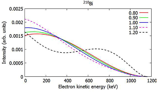
Figure 10. Normalized ISM-computed electron spectrum for the first-forbidden non-unique β− decay of 210Bi. The value gV = 1.0 was assumed and the color coding represents the value of gA.
In Kostensalo and Suhonen [71] a modest gA dependence was reported in the spectra of the decays 93Y(1/2−) → 93Zr(1/2+) and 138Cs(3−) → 138Ba(3+), as can bee seen in Figure 11. In the spectrum on 93Y some dependence on the value of ϵMEC is also seen, which opens up the possibility for investigating the mesonic enhancement of the axial-charge matrix element using the SSM.
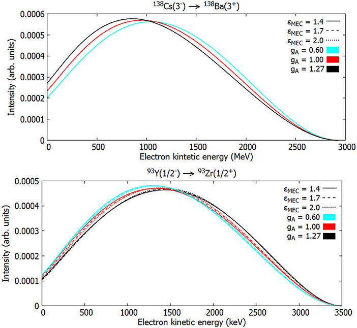
Figure 11. Normalized ISM-computed electron spectra for the first-forbidden non-unique β− decays of 138Cs and 93Y. The value gV = 1.0 was assumed and the color coding represents the value of gA and the dash coding the value of the mesonic enhancement factor ϵMEC.
Concerning the lighter nuclei, so far there are not any good candidates yet discovered. However, our recent shell-model calculation in the full fp shell using the interaction gxpf1a [79, 80] shows that the second-forbidden ground-state-to-ground-state decay of 59Fe possesses the necessary gA dependence, as can be seen from Figure 12. The branching ratio on the other hand is only 0.18 % [81], which complicates the measurement of this spectrum to the required precision. In any case, this discovery gives us hope that there might be some good candidates for the SSM also in this mass region.
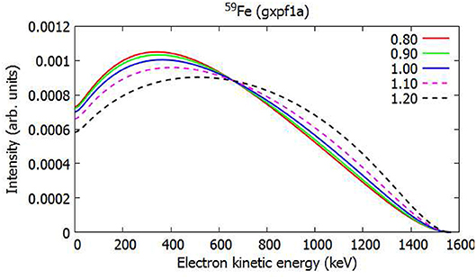
Figure 12. Normalized ISM-computed electron spectrum for the second-forbidden non-unique β− decay of 59Fe. The value gV = 1.0 was assumed and the color coding represents the value of gA.
The main issue with the SSM is the quality of the theoretical wave functions. However, the spectral shapes have been found to depend very little on the details of the wave functions making it possibly a very robust tool [49, 78]. The best candidates for the SSM found so far are, unfortunately, decay transitions between mid-shell nuclei, such as 113Cd, which are not easy to describe theoretically. Even though the SSM seems to be robust, in order to make strong claims about the effective value of gA it would be preferable to have precise wave functions. In the case of the β−-decay transition 98Tc(6+) → 98Ru(4+) our recent calculations using the glepn interaction [70] have given results which are in good agreement with the available spectroscopic data. For the 2+ state in 98Ru the calculated magnetic dipole moment +0.445μN is in agreement with the experimental value +0.8(6)μN [82] and the electric quadrupole moment −0.129e2b agrees with the experimental value -0.03(14)e2b [83] also. The interaction also manages to predict that the 4+, 5+, 6+ states in 98Tc are below 70 keV, though does not get the ordering quite right. Furthermore, the experimental half-life of the β decay is reproduced with a reasonable gA = 0.96. In comparison, the calculation carried out in Kostensalo and Suhonen [77], using the interaction by Gloeckner [84], fails to reproduce the half-life 4.2(3) × 106 yr with any effective value of gA giving 2.1 × 10⁶ yr for gA = 1.04 and less for all other values. As can be seen from Figure 13 the two Hamiltonians still predict very similar spectral shape evolution regardless of the failures in half-life prediction.
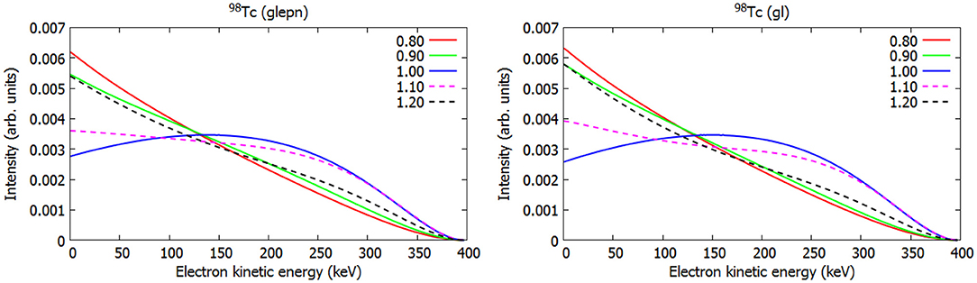
Figure 13. Normalized ISM-computed electron spectra for the second-forbidden non-unique β− transition 98Tc(6+) → 98Ru(4+) using two different Hamiltonians. The branching to this decay channel is 100%. The value gV = 1.0 was assumed and the color coding represents the value of gA.
On the experimental side advances have been made by measuring the 113Cd spectrum to high accuracy [85]. When compared with the spectral shapes given in Haaranen et al. [48] the following effective values of gA were obtained
which are in excellent agreement with each other.
4.3.2. Higher-Forbidden Unique Decays
Early studies of the quenching in the second- and third-forbidden unique β decays were performed in Towner et al. [75] and Warburton et al. [86]. In Towner et al. [75] the suppression mechanism of the first-forbidden and third-forbidden β decays of light nuclei (A ≤ 50) was studied by using simple shell-model estimates and first-order perturbation theory. The hindrance of the decay transitions was argued to result from the repulsive T = 1 (isospin 1) particle-hole force. In Warburton et al. [86] the second- and third-forbidden unique β decays were studied using a simple interacting shell model and the unified model (deformed shell model) for six β transitions in the A = 10, 22, 26, 40 nuclei. The incentive for the studies was the hindrance of certain measured β transitions. A later study of second-forbidden unique β decays in the mass range A = 10 − 54 was performed in Martínez-Pinedo and Vogel [87] by using the ISM. A reasonable correspondence with the measured half-lives was achieved by using the free value of the axial coupling but a quenched value would have improved the correspondence.
The quenching related to the virtual β transitions of the 0νββ decay can be studied at the low-q limit (5) by using the theoretical machinery of section 4.1. In Kostensalo and Suhonen [88] this machinery was applied to 148 potentially measurable second-, third-, fourth-, fifth-, sixth- and seventh-forbidden unique beta transitions. The calculations were done using realistic single-particle model spaces and G-matrix-based microscopic two-body interactions. The results of Kostensalo and Suhonen [88] could shed light on the magnitudes of the NMEs corresponding to the high-forbidden unique 0+ ↔ Jπ = 3+, 4−, 5+, 6−, 7+, 8− virtual transitions taking part in the 0νββ decays.
In the work of Kostensalo and Suhonen [88] the expected half-lives of the studied β-decay transitions were derived by comparison with the analyses performed for the Gamow-Teller and first-forbidden unique β transitions in the works [38, 76]. An example of such predictions is given in Figure 14. In the figure one sees that the expected half-lives are very long and hard to measure. On the β− side the fourth-forbidden and seventh-forbidden decay transitions are masked by the strong β− branches to the excited states of 136Ba.
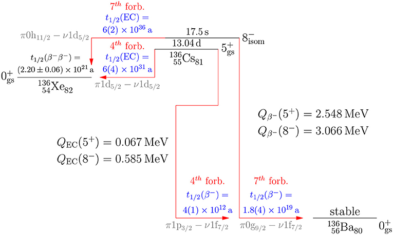
Figure 14. Predicted half-lives and their error estimates (in parenthesis) for β− and EC (electron-capture) transitions in the isobaric chain A = 136. The spin-parity assignment, life-time and decay energies (Q values) of the 5+ ground (gs) state and 8+ isomeric (isom) state of 136Cs are experimental data and taken from ENSDF [89]. The 2νββ half-life is taken from Barabash [90]. In addition to the predicted half-lives the degree of forbiddenness and the leading single-particle transition are shown.
5. Conclusions
Double β decay is a hot issue in modern day's particle, neutrino and nuclear physics. To gain the full benefit from the potential results of the running and future ββ-decay experiments, accurate evaluation of the involved nuclear matrix elements is crucial. This evaluation calls for reliable nuclear many-body approaches in order to produce realistic wave functions for ββ calculations. Beyond this, systematic estimation of the effective value of the weak axial coupling, gA, is necessary. The value of this coupling plays a notable role in both the two-neutrino and neutrinoless ββ decays.
The effective value of gA can be studied at low momentum-exchange limit by using data on β and two-neutrino ββ decays. Data on Gamow-Teller 0+ ↔ 1+ β transitions are relatively abundant and the most clean-cut to compare with calculations, thus enabling systematic studies of the quenching of gA within different nuclear-structure frameworks. The β-decay analyses (see Figure 8) suggest that effective values for masses A ≤ 82, around in the mass A = 98 − 110 region, around in the mass A = 112 − 124 region and close to for the masses A = 126 − 142 are appropriate.
Available data on first-forbidden unique β decays offer a straightforward systematic way to access the quenching of gA beyond the allowed β decays. A recent analysis (see section 4.2.2) suggests . A more involved analysis has to be performed for the first-forbidden non-unique β decays owing to the meson-exchange enhancement of the weak axial charge, combined with the quenching of gA. A recent study (see Figure 9) suggests enhancement factors ϵMEC obeying the simple linear law of Equation (43) all through the mass region A = 16 − 208. Higher-forbidden non-unique β transitions offer yet another way to study, at low-momentum-transfer limit, the quenching of gA in virtual transitions to high-angular-momentum intermediate states in the neutrinoless ββ decay. In particular, the shapes of electron spectra in these transitions can, in selected cases and once more experimental data are available, offer a viable alternative to access the quenching of gA. Here a study, combining theory with data of a recent experiment, suggests values around for the 4th-forbidden β decay of 113Cd (see Equations (52)–(54)).
Data Availability
The datasets generated for this study are available on request to the corresponding author.
Author Contributions
All authors listed have made a substantial, direct and intellectual contribution to the work, and approved it for publication.
Funding
This work has been partially supported by the Academy of Finland under the Academy project no. 318043. JK acknowledges the financial support from Jenny and Antti Wihuri Foundation.
Conflict of Interest Statement
The authors declare that the research was conducted in the absence of any commercial or financial relationships that could be construed as a potential conflict of interest.
Footnotes
1. ^Without the allowed Fermi Ji → Jf = Ji transitions.
References
1. Suhonen J, Civitarese O. Weak interaction and nuclear structure aspect of nuclear double beta decay. Phys Rep. (1998) 300:123–214. doi: 10.1016/S0370-1573(97)00087-2
2. Suhonen J, Civitarese O. Review of the properties of the 0νβ−β− nuclear matrix elements. J Phys G Nucl Part Phys. (2012) 39:124005. doi: 10.1088/0954-3899/39/12/124005
3. Engel J, Menendez J. Status and future of nuclear matrix elements for neutrinoless double beta decay: a review. Rep Prog Phys. (2017) 60:046301. doi: 10.1088/1361-6633/aa5bc5
4. Suhonen J, Civitarese O. Double-beta-decay nuclear matrix elements in the QRPA framework. J Phys G Nucl Part Phys. (2012) 39:085105. doi: 10.1088/0954-3899/39/8/085105
5. Caurier E, Nowacki F, Poves A. Shell model description of the ββ decay of 136Xe. Phys Lett B. (2012) 711:62–4. doi: 10.1016/j.physletb.2012.03.076
6. Horoi M, Neacsu A. Shell model predictions for 124Sn double-β decay. Phys Rev C. (2016) 93:024308. doi: 10.1103/PhysRevC.93.024308
7. Iwata Y, Shimizu N, Otsuka T, Utsuno Y, Menéndez J, Honma M, et al. Large-scale shell-model analysis of the neutrinoless ββ decay of 48Ca. Phys Rev lett. (2016) 116:112502. doi: 10.1103/PhysRevLett.116.112502
8. Barea J, Kotila J, Iachello F. Nuclear matrix elements for double-β decay. Phys Rev C. (2013) 87:014315. doi: 10.1103/PhysRevC.87.014315
9. Feynman RP, Gell-Mann M. Theory of the fermi interaction. Phys Rev. (1958) 109:193–8. doi: 10.1103/PhysRev.109.193
10. Patrignani C, Agashe K, Aielli G, Amsler C, Antonelli M, Asner DM, et al. (Particle Data Group). Review of particle physics. Chin Phys C. (2016) 40:100001. doi: 10.1088/1674-1137/40/10/100001
11. Šimkovic F, Pantis G, Vergados JD, Faessler A. Additional nucleon current contributions to neutrinoless double β decay. Phys Rev C. (1999) 60:055502. doi: 10.1103/PhysRevC.60.055502
12. Menéndez J, Gazit D, Schwenk A. Chiral two-body currents in nuclei: Gamow-Teller transitions and neutrinoless double-beta decay. Phys Rev Lett. (2011) 107:062501. doi: 10.1103/PhysRevLett.107.062501
13. Suhonen J. Value of the axial-vector coupling strength in β and ββ decays: a review. Front Phys. (2017) 5:55. doi: 10.3389/fphy.2017.00055
14. Ejiri H, Suhonen J, Zuber K. Neutrino-nuclear responses for astro-neutrinos, single beta decays and double beta decays. Phys Rep. (in press). doi: 10.1016/j.physrep.2018.12.001
15. Suhonen J. From Nucleons to Nucleus: Concepts of Microscopic Nuclear Theory. Theoretical and Mathematical Physics. Berlin: Springer (2007).
16. Toivanen J, Suhonen J. Renormalized proton-neutron QRPA and its application to double beta decay. Phys Rev Lett. (1995) 75:410–3. doi: 10.1103/PhysRevLett.75.410
17. Toivanen J, Suhonen J. Study of several double-beta-decaying nuclei using the renormalized proton-neutron quasiparticle random-phase approximation. Phys Rev C. (1997) 55:2314–23. doi: 10.1103/PhysRevC.55.2314
18. Vogel P, Zirnbauer MR. Suppression of the two-neutrino double-beta decay by nuclear-structure effects. Phys Rev Lett. (1986) 57:3148–51. doi: 10.1103/PhysRevLett.57.3148
19. Civitarese O, Faessler A, Tomoda T. Suppression of the two-neutrino double β decay. Phys Lett B (1987) 194:11–14. doi: 10.1016/0370-2693(87)90760-X
20. Suhonen J, Faessler A, Taigel T, Tomoda T. Suppression of the β+ decays of 148Dy, 150Er and 152Yb. Phys Lett B. (1988) 202:174–8. doi: 10.1016/0370-2693(88)90002-0
21. Suhonen J, Taigel T, Faessler A. pnQRPA calculation of the β+/EC quenching for several neutron-deficient nuclei in mass regions A = 94 − 110 and A = 146 − 156. Nucl Phys A. (1988) 486:91–117. doi: 10.1016/0375-9474(88)90041-3
22. Kortelainen M, Suhonen J. Nuclear matrix elements of 0νββ decay with improved short-range correlations. Phys Rev C. (2007) 76:024315. doi: 10.1103/PhysRevC.76.024315
23. Šimkovic F, Faessler A, Rodin V, Vogel P, Engel J. Anatomy of the 0νββ nuclear matrix elements. Phys Rev C. (2008) 77:045503. doi: 10.1103/PhysRevC.77.045503
24. Šimkovic F, Rodin V, Faessler A, Vogel P. 0νββ and 2νββ nuclear matrix elements, quasiparticle random-phase approximation, and isospin symmetry restoration. Phys Rev C. (2013) 87:045501. doi: 10.1103/PhysRevC.87.045501
25. Hyvärinen J, Suhonen J. Nuclear matrix elements for 0νββ decays with light or heavy Majorana-neutrino exchange. Phys Rev C. (2015) 91:024613. doi: 10.1103/PhysRevC.91.024613
26. Suhonen J. Calculation of allowed and first-forbidden beta-decay transitions of odd-odd nuclei. Nucl Phys A. (1993) 563:205–24. doi: 10.1016/0375-9474(93)90602-T
27. Nabi JU, Cakmak N, Stoica S, Iftikhar Z. First-forbidden transitions and stellar β-decay rates of Zn and Ge isotopes. Phys Scr. (2015) 90:115301. doi: 10.1088/0031-8949/90/11/115301
28. Nabi JU, Cakmak N, Iftikhar Z. First-forbidden β-decay rates, energy rates of β-delayed neutrons and probability of β-delayed neutron emissions for neutron-rich nickel isotopes. Eur Phys J A. (2016) 52:5. doi: 10.1140/epja/i2016-16005-6
29. Toivanen J, Suhonen J. Microscopic quasiparticle-phonon description of odd-A Xe isotopes. J Phys G Nucl Part Phys. (1995) 21:1491–7. doi: 10.1088/0954-3899/21/11/007
30. Toivanen J, Suhonen J. Microscopic quasiparticle-phonon description of odd-mass 127−133Xe isotopes and their β decay. Phys Rev C. (1998) 57:1237–45. doi: 10.1103/PhysRevC.57.1237
31. Iachello F, Van Isacker P. The Interacting Boson-Fermion Model. Cambridge: Cambridge University Press (1991).
32. Hardy JC, Towner IS, Koslowsky VT, Hagberg E, Schmeing H. Superallowed 0+ → 0+nuclear β-decays: a critical survey with tests of CVC and the standard model. Nucl Phys A. (1990) 509:429–60. doi: 10.1016/0375-9474(90)90086-2
33. Stoica S, Mirea M, Nitescu O, Nabi JU, Ishfaq M. New phase space calculations for β-decay half-lives. Adv High Energy Phys. (2016) 2016:8729893. doi: 10.1155/2016/8729893
34. Audi G, Kondev FG, Wang M, Pfeiffer B, Sun X, Blachot J, et al. The NUBASE2012 evaluation of nuclear properties. Chin Phys C. (2012) 36:1157–2014. doi: 10.1088/1674-1137/36/12/001
35. Jokiniemi L, Ejiri H, Frekers D, Suhonen J. Neutrinoless ββ nuclear matrix elements using isovector spin-dipole Jπ = 2− data. Phys Rev C. (2018) 98:024608. doi: 10.1103/PhysRevC.98.024608
36. Pirinen P, Suhonen J. Systematic approach to β and 2νββ decays of mass A = 100 − 136 nuclei. Phys Rev C. (2015) 91:054309. doi: 10.1103/PhysRevC.91.054309
37. Deppisch FF, Suhonen J. Statistical analysis of β decays and the effective value of gA in the proton-neutron quasiparticle random-phase approximation framework. Phys Rev C. (2016) 94:055501. doi: 10.1103/PhysRevC.94.055501
38. Ejiri H, Suhonen J. GT neutrino-nuclear responses for double beta decays and astro-neutrinos. J Phys G Nucl Part Phys. (2015) 42:055201. doi: 10.1088/0954-3899/42/5/055201
39. Suhonen J. Impact of the quenching of gA on the sensitivity of 0νββ experiments. Phys Rev C. (2017) 96:055501. doi: 10.1103/PhysRevC.96.055501
40. Faessler A, Lisi E, Fogli GL, Rodin V. Overconstrained estimates of neutrinoless double beta decay within the QRPA. J Phys G Nucl Part Phys. (2008) 35:075104. doi: 10.1088/0954-3899/35/7/075104
41. Suhonen J, Civitarese O. Single and double beta decays in the A = 100, A = 116 and A = 128 triplets of isobars. Nucl Phys A. (2014) 924:1–23. doi: 10.1016/j.nuclphysa.2014.01.004
42. Martínez-Pinedo G, Poves A, Caurier E, Zuker AP. Effective gA in the pf shell. Phys Rev C. (1996) 53:R2602–5. doi: 10.1103/PhysRevC.53.R2602
43. Kumar V, Srivastava PC, Li H. Nuclear β−-decay half-lives for fp and fpg shell nuclei. J Phys G Nucl Part Phys. (2016) 43:105104. doi: 10.1088/0954-3899/43/10/105104
44. Siiskonen T, Hjorth-Jensen M, Suhonen J. Renormalization of the weak hadronic current in the nuclear medium. Phys Rev C. (2001) 63:055501. doi: 10.1103/PhysRevC.63.055501
45. Behrens H, Bühring W. Electron Radial Wave Functions and Nuclear Beta Decay. Oxford: Clarendon (1982).
46. Mustonen MT, Aunola M, Suhonen J. Theoretical description of the fourth-forbidden non-unique β decays of 113Cd and 115In. Phys Rev C. (2006) 73:054301. doi: 10.1103/PhysRevC.73.054301
47. Haaranen M, Srivastava PC, Suhonen J. Forbidden nonunique β decays and effective values of weak coupling constants. Phys Rev C. (2016) 93:034308. doi: 10.1103/PhysRevC.93.034308
48. Haaranen M, Kotila J, Suhonen J. Spectrum-shape method and the next-to-leading-order terms of the β-shape factor. Phys Rev C. (2017) 95:024327. doi: 10.1103/PhysRevC.95.024327
49. Kostensalo J, Haaranen M, Suhonen J. Electron spectra in forbidden β decays and the quenching of the weak axial-vector coupling constant gA. Phys Rev C. (2017) 95:044313. doi: 10.1103/PhysRevC.95.044313
51. Ydrefors E, Mustonen MT, Suhonen J. MQPM description of the structure and beta decays of the odd A=95,97 Mo and Tc isotopes. Nucl Phys A. (2010) 842:33–47. doi: 10.1016/j.nuclphysa.2010.04.005
52. Zhi Q, Caurier E, Cuenca-García JJ, Langanke K, Martínez-Pinedo G, Sieja K. Shell-model half-lives including first-forbidden contributions for r-process waiting-point nuclei. Phys Rev C. (2013) 87:025803. doi: 10.1103/PhysRevC.87.025803
53. Warburton EK. First-forbidden β decay in the lead region and mesonic enhancement of the weak axial current. Phys Rev C. (1991) 44:233–60. doi: 10.1103/PhysRevC.44.233
54. Warburton EK, Towner IS. Renormalization of the axial charge at A ≈ 132. Phys Lett B. (1992) 294:1–6. doi: 10.1016/0370-2693(92)91629-N
55. Gove NB, Martin MJ. Log-f tables for beta decay. Atomic Data Nucl Data Tables. (1971) 10:205–19. doi: 10.1016/S0092-640X(71)80026-8
57. Kubodera K, Delorme J, Rho M. Axial currents in nuclei. Phys Rev Lett. (1978) 40:755–8. doi: 10.1103/PhysRevLett.40.755
58. Kubodera K, Rho M. Axial-charge transitions in heavy nuclei and in-medium effective chiral lagrangians. Phys Rev Lett. (1991) 67:3479–82. doi: 10.1103/PhysRevLett.67.3479
59. Kirchbach M, Riska DO, Tsushima K. The axial exchange charge operator and the nucleon-nucleon interaction. Nucl Phys A. (1992) 542:616–30. doi: 10.1016/0375-9474(92)90260-Q
60. Towner IS. Enhancement in axial-charge matrix elements from meson-exchange currents. Nucl Phys A. (1992) 542:631–58. doi: 10.1016/0375-9474(92)90261-H
61. Towner IS, Khanna FC. Role of 2p-2h states in weak 0+ − 0− transitions in A = 16 nuclei. Nucl Phys A. (1981) 372:331–48. doi: 10.1016/0375-9474(81)90039-7
62. Delorme J. Meson degrees of freedom in nuclei. Nucl Phys A. (1982) 374:541–55. doi: 10.1016/0375-9474(82)90263-9
63. Kirchbach M, Reinhardt H. On the meson-exchange correction to the axial-charge density for ns1/2 ↔n'p1/2 β-transitions. Phys Lett B. (1988) 208:79–83. doi: 10.1016/0370-2693(88)91207-5
64. Millener DJ, Alburger DE, Warburton EK, Wilkinson DH. Decay scheme of 11Be. Phys Rev C. (1982) 26:1167–85. doi: 10.1103/PhysRevC.26.1167
65. Warburton EK, Alburger DE, Millener DJ. Shapes of the 16N and 15C beta spectra and extraction of matrix elements for 15C(β−)15N(g.s.). Phys Rev C. (1984) 29:2281–9. doi: 10.1103/PhysRevC.29.2281
66. Warburton EK, Towner IS, Brown BA. First-forbidden β decay: Meson-exchange enhancement of the axial charge at A~16. Phys Rev C. (1994) 49:824–39. doi: 10.1103/PhysRevC.49.824
67. Warburton EK. Core polarization effects on spin-dipole and first-forbidden β-decay operators in the lead region. Phys Rev C. (1990) 42:2479–86. doi: 10.1103/PhysRevC.42.2479
68. Warburton EK. Mesonic enhancement of the weak axial-vector current evaluated from β decay in the lead region. Phys Rev Lett. (1991) 66:1823–6. doi: 10.1103/PhysRevLett.66.1823
69. Warburton EK. In-medium and core-polarization effects in 50K(0−) 50Ca(0+). Phys Rev C. (1991) 44:1024–9. doi: 10.1103/PhysRevC.44.1024
70. Mach H, Warburton EK, Gill RL, Casten RF, Becker JA, Brown BA, et al. Meson-exchange enhancement of the first-forbidden 96Yg(0−) → 96Zrg(0+) β transition: β decay of the low-spin isomer of 96Y. Phys Rev C. (1990) 41:226–42. doi: 10.1103/PhysRevC.41.226
71. Kostensalo J, Suhonen J. Mesonic enhancement of the weak axial charge and its effect on the half-lives and spectral shapes of first-forbidden J+ ↔ J− decays. Phys Lett B. (2018) 781:480–4. doi: 10.1016/j.physletb.2018.02.053
72. Rydström L, Blomqvist J, Liotta RJ, Pomar C. Structure of proton-deficient nuclei near 208Pb, Nucl Phys A. (1990) 512:217–40.
73. Hayen L, Kostensalo J, Severijns N, Suhonen J. First-forbidden transitions in the reactor anomaly. arXiv:1805.12259 [nucl-th] (2018).
74. Ejiri H, Ikeda K, Fujita JI. Hindrance factors for beta decays of heavy nuclei. Phys Rev. (1968) 176:1277–88. doi: 10.1103/PhysRev.176.1277
75. Towner IS, Warburton EK, Garvey GT. Hindrance phenomena in unique first- and third-forbidden β-decay. Ann Phys. (1971) 66:674–96. doi: 10.1016/0003-4916(71)90074-1
76. Ejiri H, Soukouti N, Suhonen J. Spin-dipole nuclear matrix elements for double beta decays and astro-neutrinos. Phys Lett B. (2014) 729:27–32. doi: 10.1016/j.physletb.2013.12.051
77. Kostensalo J, Suhonen J. gA-driven shapes of electron spectra of forbidden β decays in the nuclear shell model. Phys Rev C. (2017) 96:024317. doi: 10.1103/PhysRevC.96.024317
78. Kostensalo J, Suhonen J. Beta-spectrum shapes of forbidden β decays. Int J Mod Phys A. (2018) 33:1843008. doi: 10.1142/S0217751X1843008X
79. Honma M, Otsuka T, Brown BA, Mizusaki T. New effective interaction for pf-shell nuclei and its implications for the stability of the N = Z = 28 closed core. Phys Rev C. (2004) 69:034335. doi: 10.1103/PhysRevC.69.034335
80. Honma M, Otsuka T, Brown BA, Mizusaki T. Shell-model description of neutron-rich pf-shell nuclei with a new effective interaction gxpf 1. Eur Phys J A. (2005) 25:499–502. doi: 10.1140/epjad/i2005-06-032-2
81. Baglin CM. Nuclear data sheets for A = 59. Nucl Data Sheets. (2002) 95:215–386. doi: 10.1006/ndsh.2002.0004
82. Hubler GK, Kugel HW, Murnick DE. Nuclear magnetic moments of very short-lived states via the transient-field implantation perturbed-angular-correlation technique. Phys Rev C. (1974) 9:1954–64. doi: 10.1103/PhysRevC.9.1954
83. Maynard M, Palmer DC, Cresswell JR, Forsyth PD, Hall I, Martin DGE. Relative measurement of the quadrupole moments of the first excited states of the even isotopes of Ru, Pd and Cd. J Phys G Nucl Phys. (1977) 3:1735. doi: 10.1088/0305-4616/3/12/012
84. Gloeckner DH. Shell-model systematics of the zirconium and niobium isotopes. Nucl Phys A. (1975) 253:301–23. doi: 10.1016/0375-9474(75)90484-4
85. Bodenstein-Dresler L, Chu Y, Gehre D, Gössling C, Heimbold A, Herrmann C, et al. Quenching of gA deduced from the β-spectrum shape of 113Cd measured with the COBRA experiment. arXiv:1806.02254 [nucl-ex] (2018).
86. Warburton EK, Garvey GT, Towner IS. Unique second- and third-forbidden β decay. Ann Phys. (1970) 57:174–200. doi: 10.1016/0003-4916(70)90275-7
87. Martínez-Pinedo G, Vogel P. Shell model calculation of the β− and β+ partial half-lives of 54Mn and other unique second forbidden β decays. Phys Rev Lett. (1998) 81:281–4. doi: 10.1103/PhysRevLett.81.281
88. Kostensalo J, Suhonen J. Spin-multipole nuclear matrix elements in the pn quasiparticle random-phase approximation: implications for β and ββ half-lives. Phys Rev C. (2017) 95:014322. doi: 10.1103/PhysRevC.95.014322
89. ENSDF at NNDC site. Available online at: http://www.nndc.bnl.gov/
Keywords: double beta decay, Gamow-Teller beta decay, quenching of weak axial coupling, forbidden beta decay, enhancement of weak axial charge, electron spectral shapes
Citation: Suhonen J and Kostensalo J (2019) Double β Decay and the Axial Strength. Front. Phys. 7:29. doi: 10.3389/fphy.2019.00029
Received: 20 November 2018; Accepted: 18 February 2019;
Published: 19 March 2019.
Edited by:
Sabin Stoica, Horia Hulubei National Institute for R&D in Physics and Nuclear Engineering (IFIN-HH), RomaniaReviewed by:
Chandan Hati, UMR6533 Laboratoire de Physique de Clermont (LPC), FranceJameel-Un Nabi, Ghulam Ishaq Khan Institute of Engineering Sciences and Technology, Pakistan
Copyright © 2019 Suhonen and Kostensalo. This is an open-access article distributed under the terms of the Creative Commons Attribution License (CC BY). The use, distribution or reproduction in other forums is permitted, provided the original author(s) and the copyright owner(s) are credited and that the original publication in this journal is cited, in accordance with accepted academic practice. No use, distribution or reproduction is permitted which does not comply with these terms.
*Correspondence: Jouni Suhonen, am91bmkuc3Vob25lbkBwaHlzLmp5dS5maQ==