Spreading of Failures in Small-World Networks: A Connectivity-Dependent Load Sharing Fibre Bundle Model

A rich variety of multicomponent systems operating under parallel loading may be mapped on and then examined by employing a family of the Fiber Bundle Models. As an example, we consider a system composed of N immobile units located in nodes of a network $\mathcal{G}$ and subjected to a growing external load F imposed uniformly on the units. Each unit, characterized by a load threshold δ, is classified as reliable or irreversibly failed, depending on whether δ is bigger, or respectively smaller, than the load felt by the unit. A pair of interdependent units is uniquely indicated by an edge of $\mathcal{G}$. Initially all the units are reliable. When a unit fails, its load is distributed locally among interdependent neighbors if they are reliable, or is otherwise shared globally by all the reliable units. Because of the growing F and the loads that are transferred according to such a see-saw switch between the local and global sharing rules (sLGS), a set of nodes, that holds the reliable units, evolves as $\mathcal{G}\to \mathrm{\varnothing }$. During the evolution, a subset ${\mathcal{G}}_c\subset \mathcal{G}$ emerges that represents the limiting state of the system’s functionality when the smallest group of $n_c$ reliable units sustains the highest load $F_c$. We concentrate on how the Fiber Bundle Model and switching Local-Global-Sharing conspire to drive the system toward ${\mathcal{G}}_c$. Specifically, we assume that ${\left\{\delta \right\}}_{\mathcal{G}}$ are quenched-random quantities distributed uniformly over $\left(\mathrm{0,1}\right)$ or governed by the Weibull distribution and networks $\mathcal{G}$ are the Watts-Strogatz “small-world” graphs with the rewiring probability p that characterizes possible rearrangements of edges in $\mathcal{G}$. We have identified a range of values of p, where the mean highest load $f_c\left(N\right)=\langle F_c\rangle /N$, supported by reliable units, scales linearly with the average global-clustering coefficient of the host network. Similar scaling holds for $\langle n_c\rangle$ and $\langle F_c/n_c\rangle$. We have also found that in the large N limit $f_c\left(N\right)\to f_c^{\infty }>0$, for all values of p and both considered distributions of ${\left\{\delta \right\}}_{\mathcal{G}}$. The symbol $\langle \dots \rangle$ represents averaging over ${\left\{\delta \right\}}_{\mathcal{G}}$ and a suitable ensemble of networks $\left\{\mathcal{G}\right\}$.

Introduction

Numerous systems, encountered in nature as well as in different areas of science and technology, are multicomponent, i.e., they are composed of a great number of functionally identical units. When loaded, the units process a given task in a fully parallel manner. It happens, however, that a unit becomes overloaded and fails. Its load has to be undertaken by other units, which in turn may trigger subsequent overloading followed by resulting failures. Such a chain of failures gradually degrades the system performance and leads to an avalanche of failures. It may even happen that the avalanche becomes self-sustained giving rise to a catastrophe which overwhelms all the units. Different factors characterize a given system. This is important to identify those working together that push the system toward the catastrophic avalanche.

The Fiber Bundle Model (FBM) is a particular case of a wide class of cascading processes on networks [1]. It offers a flexible approach to study how multicomponent systems evolve under varying load [2–8]. The flexibility refers to such aspects as: a) range and symmetry of interactions among units [9], b) rate of load’s variation, c) heterogeneity/uniformity of units [10, 11]), or d) varying quality of units [12, 13], to name a few. The aspects a) and b) especially refer to ingredients of the FBM that play a major role when a given system is mapped onto a bundle of interacting fibers [14]. Exemplary problems, from an ample set of systems expressed in the FBM framework, cover research fields that span from geophysics including earthquakes, snow or landslides, to technology with electrical and mechanical engineering systems.

In this context, we consider a toy model of failures spreading in a set of interconnected units. Our model consists of N units that reside at nodes of an undirected simple graph $\mathcal{G}$ whose edges represent pairs of interdependent units. The units are either reliable or irreversibly failed, and we assume that an externally applied load F is distributed identically on all reliable units. When F starts growing, some units begin to suffer from insufficient strength to bear the load and they fail. Their loads remain in the system and are shared either by the nearest neighboring units, if they are reliable, or by all other reliable units. If on a given node a failure emerges, this node is removed from the graph together with corresponding edges, i.e., $\mathcal{G}$ is reduced to ${\mathcal{G}}^{\prime }\subset \mathcal{G}$. This means that under growing F, an initially connected $\mathcal{G}$ evolves toward the empty graph. In other words, unbounded growth of F pushes the set of reliable units to extinction. If the growth of F is sufficiently slow, then a distinct group of reliable units may be selected in the course of evolution:

${\mathcal{G}}_0\supset \mathcal{G}\left(F>0\right)\supset \mathcal{G}(F^{\prime }>F)\supset \dots \supset \mathcal{G}(F_c>\dots >F)\to \mathrm{\varnothing }(1)$

This group, identified by nodes of ${\mathcal{G}}_c=\mathcal{G}\left(F_c\right)$, is the smallest group of units that remain reliable under the highest load $F_c$, i.e., a load $F>F_c$ will trigger an ultimate, self-sustained avalanche of failures that overwhelms the entire system. The chain of inclusions 1 displays graphs that are stable under consecutive values of F whereas intermediate graphs, induced exclusively by loads sharing processes to be precise, are omitted for the sake of simplicity. We use the subscripts “c” to mark that the load $F_c$ is critical to the systems and that ${\mathcal{G}}_c$ represents the smallest non-empty stable configuration that precedes extinction. We call this configuration the critical configuration.

Within this work we are interested in questions like: how small a group of units can be and/or to what extent we can apply the external load while still preventing the extinction of reliable units. Subsequently, we apply the FBM to study evolving failure on “small-world” networks that are omnipresent in life and technology. Specifically, we will focus on a family of random graphs generated by the Watts-Strogatz model [15]. The reason is that such graphs reveal short average path lengths and high clustering that are key features of social networks [16].

Model Description

Take a locally overloaded system which detects a failure of a unit. In the first instance the system attempts to solve the problem locally by distributing the load among nearest neighbors of the failed unit. If such a neighborhood does not exist, the entire set of reliable units is engaged into sharing the load from the unit being lost. Such a mode of load transfer yields a significant impact on the system’s strength. Whenever an island of reliable units emerges during the evolution, its terminal load is shared globally by the system. This means that the net load transferred to reliable units that are located on the outer island’s perimeter is lower than it would be if the local load sharing (LLS) rule has been in operation. In consequence, the switching Local-Global-Sharing (sLGS) mitigates the expansion of a dominantly large cluster (DLC) of failed units and thus, the strength of the system becomes higher than that one corresponding to the LLS rule [5].

In the following, we consider an ensemble of units assigned to nodes of a graph $\mathcal{G}$ and characterized by quenched load thresholds ${\left\{\delta \right\}}_{\mathcal{G}}$. Each unit, initially considered reliable, either stays reliable or switches irreversibly to failed if the load, acting on the unit becomes higher than corresponding δ. Units are not perfect and differ in their efficiency to sustain the load. Hence, the corresponding δs are different. For the sake of simplicity we assume that ${\left\{\delta \right\}}_{\mathcal{G}}$ are quench-random quantities. We employ two distributions, assuming that thresholds are: i) uniformly distributed over the segment $\left(\mathrm{0,1}\right)$ or ii) assigned according to the Weibull pdf. Specifically, the second distribution is employed to analyze networks with components of technological nature.

Watts-Strogatz Model and Small-World Networks

There exists an ample set of papers that discuss the Watts-Strogatz model in details [17]. Hence, for the purpose of our model, it is sufficient to present the simplest exemplary graph and sketch how its modifications enable a smooth passage from an ordered network to disordered ones through a multitude of “small-world” graphs. One such passage is shown in Figure 1. The presented graphs are generated in two steps:

• a ring over N nodes is created and each node is connected with its k nearest neighbors, k is even.

• for every node with uniform independent probability p, each edge is rewired to a node that is selected uniformly at random while avoiding loops and edge duplication.

FIGURE 1

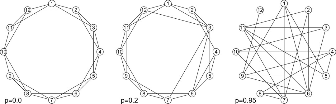
FIGURE 1. Exemplary “small-world” networks generated by the Watts-Strogatz model with mean node degree $k=4$ and growing probability p of rewiring.

These steps are illustrated in Figure 1, e.g., the first step corresponds to the graph with $p=0$. In simulations we will employ graphs with $k=4$.

Among the different characteristics of a network, one is particularly important in the view of our study, namely the global clustering coefficient C defined as:

$C=\frac{3\times \mathrm{number of triangles}}{\mathrm{number of connected triples}},(2)$

where nodes of a triangle form a 3-clique, and a connected triple is a tree.

Applying External Load

We have assumed the external load F is distributed identically on all reliable units. Consider a load $f_i$ that locally acts on i-th unit, out of M reliable ones that are present at a given stage of evolution. This $f_i$ combines $F/M$ with a load generated by shared loads agglomerated from previous failures that affected other units. An important feature of such a process is that the shared loads transferred from failed units and the externally applied load may together activate bursts of subsequent failures. The bursts may become self-sustained and they either eliminate all the reliable units or they cease and freeze the system in a stable configuration.

We consider a configuration $\mathcal{G}\left(F\right)$ being stable, if under a given F all reliable units keep their states unchanged. When no reliable unit exists the corresponding configuration is the empty graph $\mathrm{\varnothing }$. Along with this notation, ${\left\{f\left(F_t\right)\right\}}_{\mathcal{G}\left(F_t\right)}$ is the pattern of load detected locally at nodes of $\mathcal{G}\left(F_t\right)$.

In order to identify $F_c$, along with the size of the smallest set of reliable units, we increase the load stepwise, according to the method known as quasi-static loading. In detail, when $F=0$ all units are reliable and the initial configuration is stable. Consecutive load steps are adjusted according to the rule: if $F_t>0$ and the system attains a stable configuration $\mathcal{G}\left(F_t\right)$, then $F_{t+1}=F_t+\text{min}\left[{\left\{f\left(F_t\right)-\delta \right\}}_{\mathcal{G}\left(F_t\right)}\right]$ will either drive the system to another stable configuration $\mathcal{G}\left(F_{t+1}\right)$ or initiate an avalanche of failures that destroys all still reliable units, i.e., the system reaches the configuration $\mathrm{\varnothing }$.

From this, we derive the stopping rule:

$\mathcal{G}\left(F_t\right)\ne \varnothing \wedge \mathcal{G}\left(F_{t+1}\right)=\varnothing \Rightarrow F_t=F_c\wedge n_c=\left|\mathcal{G}\left(F_c\right)\right|(3)$

where $n_c=\left|\mathcal{G}\left(F_c\right)\right|$ is the size of $\mathcal{G}\left(F_c\right)$, i.e., the size of the smallest group of reliable units. We use this rule in simulations.

Load Sharing Rule

The load transfer requires a rule that indicates how a load released by a failure is shared by other reliable units. We define our rule in a following way: the reliable network neighbors are obliged to equally share the load if they are accessible and all the reliable units acquire the load in the contrary case.

From this definition’s point of view, our rule “dynamically” switches between two rules, which are known in the FBM framework as global load sharing (GLS) and LLS. These rules correspond to two extremal ranges of load transfer. In the GLS rule, a load originating from a failed unit is transferred equally to all the reliable units and thus, the range of transfer is maximal. The LLS rule, in turn, engages only the nearest neighbors of a node that fails, so the range of load transfer is minimal. As a consequence, the load distributed according to the GLS rule is the least harmful for the system, whereas the LLS represents the most damaging method of the load distribution.

In simulations, we call this rule the sLGS and assume that the load transfer is an almost instantaneous process that happens simultaneously. We can mathematically express the sLGS in a framework for cascading processes on networks [18]. For this purpose, let ${\widehat{A}}_{\mathcal{G}}$ be the adjacency matrix of $\mathcal{G}$, whose nonzero entries $A_{\mathcal{G}}^{ij}=1$ appear only if the units i and j are interdependent and let $k_i={{{\displaystyle \sum }}^{\text{}}}_{j\ne i}^{\left|\mathcal{G}\right|}{A}_{\mathcal{G}}^{ij}$ denotes the degree of node i at the stage $t_{\mathcal{G}}$ of evolution characterized by $\mathcal{G}$. With this notation, a fraction of load $f_i$ transferred from the failed unit i to a reliable unit j reads

$\text{Δ}{f}_{j\leftarrow i}=\left[A_{\mathcal{G}}^{ij}\cdot \frac{1}{k_i}+\left(1-A_{\mathcal{G}}^{ij}\right)\frac{1}{\left|\mathcal{G}\right|-n_{\mathcal{G}}}\right]\cdot f_i,(4)$

where $n_{\mathcal{G}}$ represents the number of nodes that fail at the stage $t_{\mathcal{G}}$ and are not neighbors to site i.

Equation 4 has a structure that resembles schemes of load transfer known from the literature. Namely the mixed-mode load sharing (MMLS) [19] and the heterogeneous load sharing (HLS) [20] merge together the LLS and the GLS in order to study a crossover behavior in FBM on regular lattices. The MMLS employs a constant quota q to split each transferred load into two streams: a portion q of the load goes to nearest neighbors under the LLS rule and the remaining portion is transferred according to the GLS rule. Thereby, the MMLS folds the LLS and the GLS in a manner that both rules are simultaneously activated in each failure. This is in contrast to the HLS, which in turn assigns units to two groups in order to discriminate between units located in “rigid nodes” and those residing in a “flexible” fraction of the support. If the “rigid” unit fails then the GLS transfers its load whereas the LLS governs the transfer from the “flexible” unit. The MMLS and the HLS are static, i.e., the corresponding values of q and sets of nodes at which q-weighted sharing rules operate are chosen and fixed prior to loadings. We also want to mention the modified LLS rule [21]. By employing the scheme $\text{Δ}{f}_{j\leftarrow i}=A_{\mathcal{G}}^{ij}\cdot \left(f_i/k_i\right)$, this rule sheds loads released from isolated clusters of failed nodes rather than transferring these loads to remaining intact parts of the system.

It is worth noting that rules, similar to the sLGS have been applied recently in such contexts as a strategy for stopping failure cascades [22] or clogging in multichannel supply systems [23].

A Range of Possible Applications

The above-described load sharing rule operating among units interconnected through a small world network may serve as a toy model of cascading failures in economy or technology. A general scenario we have in mind concerns a default initiated by an unsupported on-site demand that spreads through the system in a form of a contagion from the defaulter, either to units which are closely associated or to other ones. Clearly, when a unit switches into default this affects other units. Depending on the context, units could be: a) institutions, as, e.g., banks belonging to an interbank network, b) workers with beneficial loans from a company, borrowers in micro financial markets or c) elements of power grids, especially of small scale smart grids. With this same spirit a load could be seen as a demand, e.g., for liquidity or electric power. Below we list some basic facts that are relevant to our model.

Interbank Market

Undirected graphs are suitable to modeling interbank networks, especially in the context of a financial contagion [24, 25]. Among representations which are convenient and applied in studies, a possible one connects a pair of banks by an undirected edge whenever there exists an interbank liability or claim [25]. When an ensemble of interdependent banks is mapped onto a graph, one can analyze its static and dynamic properties. A class of small world graphs certainly is relevant in this context. It was shown, e.g., that the interbank market of $\sim 900$ Austrian banks is a small-world network [25].

Microeconomy

Many companies offer beneficial loans to its employees. Specifically, to those suffering financial troubles. These employees-debtors, being colleagues and friends, are frequently mutual guarantors and can thus be considered as members of a resulting social network.

Power Grids

The small world topology is frequently reported as present in power grid networks [26–28]. This is equally true for large scale installations involving nationwide power systems in the US or Europe as well as for medium or small power grids [29, 30]. Particularly, in smart grids of renewable energy sources, such as small-scale photovoltaic systems or small-wind turbines [31, 32], the small world topology is beneficial. For example, networks with small world connectivity can significantly enhance their robustness against different attack by simultaneous increase of the rewiring probability and average degree [33].

Results and Discussion

In order to acquire data necessary to build reliable empirical distributions, we have adopted two computational schemes that correspond to small and large numbers of units. In the first scheme, for each N, an ensemble of $M_{\delta }$ load-threshold distributions ${\left\{{\delta }_i\right\}}_{i\in \left\{1,\dots N\right\}}$ is generated. Then, for each selected value of $p\in \left[\mathrm{0,1}\right]$ a separate ensemble ${\left\{{\mathcal{G}}^{\left(s\right)}\left(N,p\right)\right\}}_{s=1,\dots ,M_{\mathcal{G}}}$ of Watts-Strogatz graphs $\mathcal{G}\left(N,p\right)$ is formed and stored. This means that for each chosen pair $\left(N,p\right)$, two corresponding ensembles ${\left\{{\delta }_i\right\}}_{i=1,\dots ,N}$ and $\mathcal{G}\left(N,p\right)$ allow us to probe $M_{\delta }\cdot M_{\mathcal{G}}$ different realizations of failure evolution for the uniform as well as for the Weibull distributions of $\left\{\delta \right\}$. To study networks with $N\le {10}^3$, we employ the first scheme with $M_{\delta }=2500$ and $M_{\mathcal{G}}=400$. The second scheme involves systems with $\mathrm{1,200}\le N\le \mathrm{21,600}$. For each chosen values of $\left(N,p\right)$, a set consisting of ${10}^4$ pairs $\left({\left\{{\delta }_i\right\}}_{i=1,\dots ,N},\mathcal{G}\left(N,p\right)\right)$ is generated. The two computational schemes allow us to probe ${10}^6$ or ${10}^4$ different realizations of failure evolution for a small or large N regime, respectively.

We use both computational schemes for uniformly distributed load thresholds. In simulations with the Weibull distribution we consider $\rho =\mathrm{2,3,5}$ and 8. For all these ρ we conduct simulation following the first computational scheme. In the large N limit, we restrict ourselves to distributions with $\rho =2$ only.

Subsequently, when averaging a quantity Y over either $\left\{\delta \right\}$ or $\left\{\mathcal{G}\right\}$ alone, we denote the respective mean by ${\overline{Y}}^{\delta }$ and ${\overline{Y}}^{\mathcal{G}}$, whereas the symbol $\langle Y\rangle$ refers to averaging Y over both ensembles.

Maximal Supported Load and Minimal Number of Reliable Units

Following the described computational schemes, we have collected large data sets containing detailed information about how the maximal load, together with the minimal number of units, vary when we pass through all pairs ${\left\{{\delta }_i\right\}}_{i=1,\dots ,N},\mathcal{G}\left(N,p\right)$ of stored ensembles.

The gathered data turn out to be skewed independently of what distribution governs $\left\{\delta \right\}$. Specifically, the data pointed to $F_c$ are positively skewed whereas the data related to $n_c$ reveal negative skewness. This can be seen in Figure 2 for chosen values of N and $p=0.2$. Interestingly, we were able to fit all data by one family of probability distributions (p.d.), namely by the three-parameter skew-normal p.d. [34] defined as:

$\varphi \left(x\right)=\frac{\text{erfc}\left(-\alpha \frac{x-\mu }{\sqrt{2}\sigma }\right)}{\sqrt{2\pi }\sigma }\text{exp}\left[-{\left(\frac{x-\mu }{\sqrt{2}\sigma }\right)}^2\right],(5)$

where μ, σ and α are the location, scale and shape parameters, respectively.

FIGURE 2

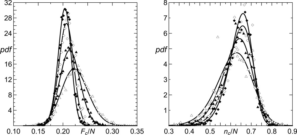
FIGURE 2. Calculated distributions of $F_c/N$ (left diagram) and $n_c/N$ (right diagram) for an increasing number of units: $N=100$ (white triangles), $N=200$ (black triangles), $N=400$ (white diamonds) and $N=600$ (black diamonds). Each value of N corresponds to a population of 2,500 load thresholds ${\left\{{\delta }_i\right\}}_{i\in \left\{1,\dots N\right\}}$ distributed uniformly over $\left(\mathrm{0,1}\right)$ and an exemplary Watts-Strogatz graph with $p=0.2$. The solid lines are drawn according to Eq. 5 with parameters estimated from the simulations.

We have rigorously examined the data sets employing a number of goodness of fit tests, including the Cramer-von Mises and Anderson-Darling tests [35] and have accepted $\varphi (\cdot )$, Eq. 5, as the distribution that best fits the empirical distributions of $F_c/N$ and $n_c/N$. A selection of correct distribution for gathered data sets is an important task. Appropriate methods exist to establish confidence sets and perform hypothesis tests, including an universal procedure [36]. In this regard we should mention that a substantial portion of our data sets is satisfactorily modeled by the three-parameter Weibull p.d. also. We opt, however, for representing all data by Eq. 5 because the skew-normal p.d. works correctly for almost all data sets and for those when both models are acceptable, the skew-normal p.d. returns higher values of maximized likelihood function and greater p-values than the Weibull p.d.

We have also estimated values of the parameters μ, σ and α. The gathered data yield estimate functional dependences of μ, σ and α on model parameters $N,p$ and ρ. As an example, consider empirical p.d. of $F_c/N$ related to different values of rewiring probability $p\in \left[\mathrm{0,1}\right]$. The corresponding skew-normal p.d. reads:

$\varphi \left(F_c/N,N,p\right)=\frac{\text{erfc}\left(-{\alpha }_F\left(N,p\right)\frac{F_c/N-{\mu }_F\left(N,p\right)}{\sqrt{2}{\sigma }_F\left(N,p\right)}\right)}{\sqrt{2\pi }{\sigma }_F\left(N,p\right)}\text{exp}\left[-{\left(\frac{F_c/N-{\mu }_F\left(N,p\right)}{\sqrt{2}{\sigma }_F\left(N,p\right)}\right)}^2\right].(6)$

We have directly written that $\mu ,\sigma$ and α are functions of N and p whereas parameters characterizing distributions of $\left\{\delta \right\}$ are omitted. We have estimated the functional dependences of these coefficients on model parameters. For instance, in Figure 3, we present how the location parameter μ varies with p, while keeping constant values of N. The resulting fitting function turns out to be a polynomial of the third order in p.

FIGURE 3

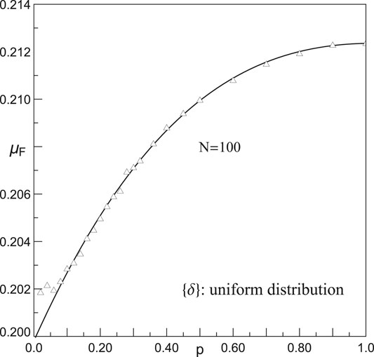
FIGURE 3. Estimated functional dependence of ${\mu }_F$ on rewiring probability p: ${\mu }_F=a+b{\left(1-c\cdot p\right)}^3$, with $a=0.2128\pm 0.0006$, b = $0.01228\pm 0.005$ and $c=0.741\pm 0.079$ for $N=100$. Each data point corresponds to averaging over ${10}^6$ samples.

Since the location parameter ${\mu }_F$ grows with p and $F_c/N$ is positively skewed $\left({\alpha }_F>0\right)$ then the corresponding mean ${\langle F\rangle }_c/N$ increases. This is because $\langle F_c\rangle /N={\mu }_F+\sqrt{2}\cdot {\alpha }_F\cdot {\sigma }_F/\sqrt{\pi \left(1+{\alpha }^2\right)}$. Similar calculations yield estimators related to $n_c$ and $F_c/n_c$. As an example, an average critical number of units $\langle n_c\rangle /N$ is presented in Figure 4 for uniformly distributed $\left\{\delta \right\}$. Data related to the Weibull distribution with exemplary values of ρ are displayed in Figure 12.

FIGURE 4

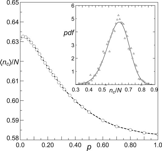
FIGURE 4. Scaled mean critical number of reliable units $\langle n_c\rangle /N$ for $N=100$. The sample size equals ${10}^6$. The Inset shows empirical distribution of $n_c/N$ computed from 2,500 uniform distributions of load thresholds for an exemplary Watts-Strogatz graph with $p=0.2$.

It should be pointed out that when p is growing, the resulting networks become more and more disordered and the probability that a given node has a low degree increases. Hence, the sLSG activates all the reliable units more frequently than it happens in networks generated with a small value of p.

Large N Limit

Even though the applications mentioned in Section 2.4 refer to networks composed of about ${10}^2–{10}^4$ units, it is worth addressing the questions on how the sLGS drives a very large system and how such the system converges to attain its ultimate strength. In the following we report relevant details.

It is known that the LLS model on a complex network behaves similarly to the GLS model giving rise to a non-vanishing critical strength $f_c$ in the large N limit [5]. Formally, the family of Wats-Strogatz graphs covers the spectrum of networks ranging from the locally regular $\left(p=0\right)$ to the maximally disordered $\left(p=1\right)$ ones. The locally regular network is the only exception in this family because under the LLS the strength $f_c$ decays as$\sim 1/\text{log}\left(N\right)$. Is this thus obvious that, the sLGS, by switching between the LLS and the GLS, does the same?

Based on results of simulations of large-N systems, we have found that: i) $f_c\to f_c^{\infty }>0$, ii) $f_c^{\infty }$ depends quantitatively on p and ${\left\{\delta \right\}}_{{\mathcal{G}}_0}$, and iii) $f_c^{\infty }$ depends qualitatively on probability distribution that generates ${\left\{\delta \right\}}_{{\mathcal{G}}_0}$. For the uniform p.d.

$f_c^u\left(z=1/\text{log}\left(N\right),p\right)\sim f_u^{\infty }\left(p\right)+A_u\left(p\right)\cdot z^{\alpha \left(p\right)}(7)$

while for the Weibull p.d. the best fit reads

$f_c^w\left(z=1/\text{log}\left(N\right),p,\rho \right)\sim f_w^{\infty }\left(p,\rho \right)+A_w\left(p,\rho \right)\cdot z+B_w\left(p,\rho \right)\cdot z^2,(8)$

where the subscripts u and w stand for the uniform and Weibull distributions, respectively. The estimated system’s strength $f_u^{\infty }$ and the exponent α are displayed in Figure 5. Correspondingly, for the Weibull p.d. $f_w^{\infty }$ is presented in Figure 6 whereas the amplitudes $A_w,B_w$ are shown in Figure 7.

FIGURE 5

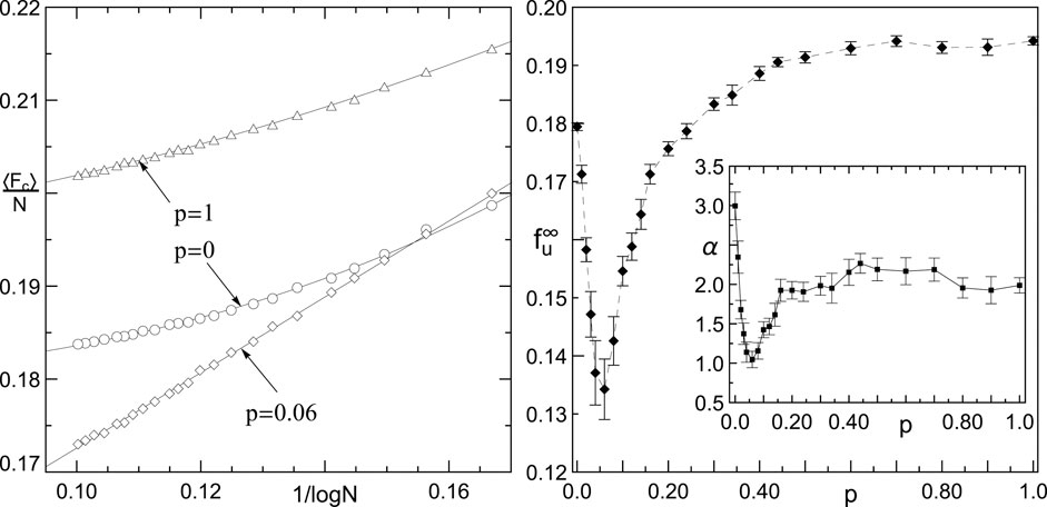
FIGURE 5. Left panel: The logarithmic size dependence of system strength for networks that: are ordered ($p=0$), disordered ($p=1$) and correspond to the weakest system ($p=0.06$). The lines are drawn following Eq. 7 with coefficients shown in the right panel. Right panel: The ultimate system strength $f_u^{\infty }$ and exponent α (Inset) computed for different values of p according to the best fit given in Eq. 7. Black marks represent the best fit to data of which some examples are shown in the left panel. The error bars indicate $95\text{\%}$ confidence intervals. Data in both panels refers to $\left\{\delta \right\}$ distributed uniformly over $\left(\mathrm{0,1}\right)$.

FIGURE 6

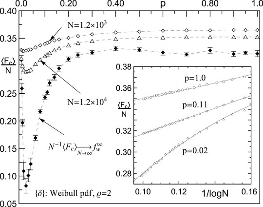
FIGURE 6. The system’s strength scaled by size in the large N limit. Inset: the logarithmic dependence of scaled system strength for: $p=0.02$ (minimum of $f_w^{\infty }$), $p=0.11$ ($B_w\sim 0\Rightarrow f_w^{\infty }\sim 1/\text{log}\left(N\right)$, see Eq. 8 and Figure 7) and $p=1$ (maximally disordered network). Data correspond to the Weibull distribution of $\left\{\delta \right\}$ with $\rho =2$. The sample size is equal to ${10}^4$ for each data point.

FIGURE 7

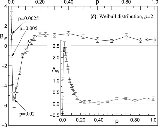
FIGURE 7. Amplitudes $A_w$ (Inset) and $B_w$ of $f_c$ in the large N limit for systems with $\left\{\delta \right\}$ governed by the Weibull p.d., see Eq. 8. Each data point results from an averaging of over ${10}^4$ samples.

These plots illustrate a variety of ways in which $f_c$ converges toward $f_c^{\infty }$. For both distributions of $\left\{\delta \right\}$, the locally regular network $\left(p=0\right)$ sustains $f_c^{\infty }>0$. For small values of p the ultimate system strength rapidly decreases, attains its minimum and then increases. Until $p\sim 0.2$ the growth of $f_c$ is fast, then moderate, until $p\sim 0.5$. For $p>0.5$ the strength varies a little and saturates around value $0.77\times f_c^{\infty }\left(GLS\right)$, where $f_c^{\infty }\left(GLS\right)$ is the ultimate strength for the GLS rule, i.e., $f_c^{\infty }\left(GLS\right)=0.25$ for uniformly distributed $\left\{\delta \right\}$ and $f_c^{\infty }\left(GLS\right)={\left(\rho \cdot \text{e}\right)}^{-1/\rho }$ for the Weibull distribution. As shown in Figure 7, except for $p\lesssim 0.003$, the amplitude $B_w$ is negative up to $0.11<p^{\text{*}}<0.12$, then becomes positive. This means that $f_c^w\left(1/\text{log}\left(N\right)\right)$ is concave down for $p<p^{\text{*}}$. Therefore, the speed of convergence of $f_c^w\left(1/\text{log}\left(N\right)\right)$ grows when $1/\text{log}\left(N\right)$ tends to zero. Passing $p^{\text{*}}$, the function $f_c^w$ becomes concave up and the speed of its convergence toward $f_w^{\infty }$ slows down.

A deep minimum of $f_u^{\infty }$ at $p\sim 0.06$, seen in Figure 5, and correspondingly that of $f_w^{\infty }$ at $p\sim 0.02$, displayed in Figure 6, result from an interplay between a slightly perturbed order of the locally regular network and the activity of the GLS-component of the sLGS rule. This can be qualitatively explained by adopting arguments formulated in [5]: (i) when a complex network is progressively loaded, the FBM with the LLS rule behaves as the GLS model because clusters of failed units appear, continuously grow and glue into a DLC, (ii) due to the small-world effect, reliable units remain closely to each other and to the DLC and thus, the system resembles the GLS model, (iii) on an ordered network which is spatially uniform, clusters of failed units originate and extend in an equal condition and the DLC emerges abruptly. Now consider the argument (iii) in conjunction with the sLGS rule engaged on a network with $p\sim 0$. Since the network is almost regular and highly clustered the LLS component prevails over the GLS one in the early stages of the loading process. The sLGS rule with its frequently activated LLS component continues operating until the network becomes fragmented. Then, the GLS component starts to allocate terminal loads from failed fragments to units that are still reliable. From there, the process behaves similarly to that with the GLS rule. Contrary to the case of the LLS rule, the resulting system strength does not vanish. It is, however, smaller than that corresponding to the GLS rule. When p increases, the arguments (i) and (ii) come into the picture. First, for $0.01\lesssim p\lesssim 0.1$, the average path length begins to decrease whereas networks are still highly clustered albeit no more locally ordered. Even that such conditions support a gradual DLC emergence, the average path length is not sufficiently small to facilitate the DLC growth. This, combined with the lack of local ordering favor the LLS component activity on clusters bigger than those appearing within an almost ordered network. In consequence, the system strength passes through its minimum. Networks with p roughly bigger than 0.1 enter a scenario characterized by the argument (i). The sLGS differs from the LLS, however. As it was already stated in the beginning of Section 2, whenever an island of reliable units appears its terminal load is transferred by the sLGS to all other reliable units and not to the closest ones. This inhibits the DLC growth and increases the system strength correspondingly.

Within our numerical approach, it is difficult to precisely estimate $f_c^{u,w}$ in the very close vicinity of $p=0$. For this reason, we were unable to analyze the continuity of $f_{u,w}^{\infty }$ when $p\to 0$. Therefore the question arises whether $f_{u,w}^{\infty }\left(p=0\right)$ is an isolated point of the ultimate system strength.

Internal vs. External Load From a Reliable-Unit’s Point of View

When considering its future reliability, a prospective unit behaves as an outer observer whose forecast is limited to the external load F. When entering the system, the unit is confronted with an internal-load impact. It is thus worth discussing to what extent these two points of view differ.

We have assumed that during the evolution, the external load F is distributed identically on reliable units and is growing stepwise along the rule that was discussed in SubSection 2.3.

Having initially ${\mathcal{G}}_0\ne \mathrm{\varnothing },F_0=0,{\left\{f\left(0\right)\right\}}_{{\mathcal{G}}_0}={\left\{0\right\}}_{{\mathcal{G}}_0}$, the rule yields consecutive $F_t$:

if $\mathcal{G}\left(F_t\right)\ne \mathrm{\varnothing }$ then

$\begin{array}{l}{F}_{t+1}=F_t+\text{min}\left[{\left\{\delta -f\left(F_t\right)\right\}}_{\text{G}\left(F_t\right)}\right]\wedge \text{G}\left(F_t\right)\to \text{G}\left(F_{t+1}\right)\subset \text{G}\left(F_t\right)\\ \mathrm{else}\\ F_c=F_t\wedge n_c=\left|\text{G}\left(F_c\right)\right|\\ \mathrm{end}\mathrm{if}\end{array}$

This iterative chain involves successive patterns of local load ${\left\{f\left(F_t\right)\right\}}_{\mathcal{G}\left(F_t\right)}$ that are strongly affected by the load-sharing rule, i.e., the mLGS in our case.

Now, consider $n_t$ units that are reliable at the stage t of the evolution. Let us choose one of them, say the i-th unit. This means that ${\delta }_i>f_i$, where $f_i$ is the local load at node i. When $F_t\to F_{t+1}>F_t$ then $n_t\to n_{t+1}<n_t$ and the pattern of local load becomes ${\left\{f\left(F_{t+1}\right)\right\}}_{\mathcal{G}\left(F_{t+1}\right)}$. The state of our chosen unit is now determined by the difference between the quenched value of ${\delta }_i$ and the updated ${\tilde{f}}_i$. While ${\delta }_i$ remains unchanged, the updated ${\tilde{f}}_i$ increases because of a growing $F_{t+1}/n_{t+1}>F_t/n_t$ and new shared loads, possibly assigned to the unit at the stage t. Clearly, internal-load distributions are subject to non-trivial variations that can be observed during the evolution.

It is important to make a distinction between impacts of external and internal loads on units. To obtain a closer look at these different impacts, we compare $F_t/n_t$ with ${\left\{f\left(F_t\right)\right\}}_{\mathcal{G}\left(F_t\right)}$ for a given network $\mathcal{G}\left(F_t\right)$ in the course of evolution. As an illustrative example, we compare the impacts at critical configuration resulting from averaging over ${10}^6$ samples. Figure 8 displays $\langle F_c\rangle /\langle n_c\rangle$ and $\langle {\left\{f\left(F_c\right)\right\}}_{{\mathcal{G}}_c}\rangle =\langle F_c/n_c\rangle$.

FIGURE 8

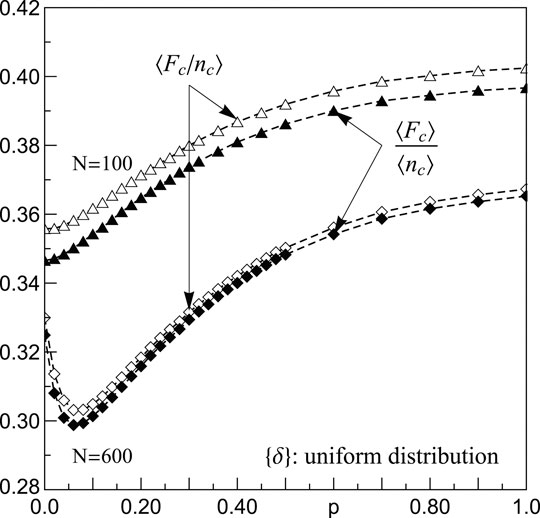
FIGURE 8. Mean critical load per reliable unit: white plot marks - internal load $\langle F_c/n_c\rangle$ and black plot marks - external load $\langle F_c\rangle /\langle n_c\rangle$. The sample size is equal to ${10}^6$ for each data point. The dashed lines are only visual guides.

Analyzing computed values, we detect that the mean internal load prevails over the mean external one for all values of p. In networks with $N\sim {10}^2$, the relative difference is of the order of 0.01 and thus, is relevant to a prospective unit. Such a difference should be taken into account when forecasting long-term reliability, especially when considering units with low values of their δs.

Small-World Properties at Critical Configuration

When the sLGS rule is in operation, a load is assigned according to accessibility of reliable units, i.e., either locally or globally. If the hosting network reveals a relatively strong local connectivity, then the sLGS looks like the LLS.

A lasting presence of reliable nearest-neighbours depends on a connectivity of an underlying network. Independently of the value of rewiring probability p, random graphs generated by the Watts-Strogatz model preserve the number of edges and mean-node degree. This means that when p grows, we pass from ordered to disordered networks, keeping the numbers of nodes and edges unchanged. For intermediate values of p, the resulting networks turn out to be locally clustered, whereas randomly rewired edges reduce the mean path lengths. Thus, there exists a range of p, where networks belonging to $\left\{{\mathcal{G}}_0\left(N,p\right)\right\}$ resemble a so-called “small-world” environment, i.e., they reveal a relatively strong clustering and a short mean path length.

We thus expect that the “small-world” properties would mark their presence in data sets related to $F_c,n_c$ and $F_c/n_c$. When analyzing the data together with values of the global clustering coefficient C, defined by the Eq. 2 and computed for corresponding networks, we notice that for a given value of N, formula

$\langle Y\rangle \left(p\right)=u+w\cdot {\left(1-\xi \cdot p\right)}^3(9)$

best fits the quantity $\langle Y\rangle$ that represents the following mean: $\langle F_c/n_c\rangle ,\langle F_c\rangle$ and $\langle n_c\rangle$. Detailed information is presented in Table 1. Because the same fit (9) also holds for ${\overline{C}}^{\mathcal{G}}\left(N,p\right)$ we can relate $\langle Y\rangle$ directly to ${\overline{C}}^{\mathcal{G}}$. Interestingly, it appears that the corresponding relation is linear for a range $p\in \left\{p_N^{-},p_N^{+}\right\}$ that depends on N, namely:

$\langle Y\rangle =a+b\cdot {\overline{C}}^{\mathcal{G}}(10)$

TABLE 1

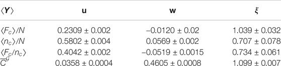
TABLE 1. Estimated coefficients in Eq. 9: $\langle Y\rangle =u+w\cdot {\left(1-\xi \cdot p\right)}^3$, for systems with $N=100$ units and uniformly distributed δs.

Figure 9 displays respective relations for systems with uniformly distributed $\left\{\delta \right\}$. Appropriate coefficients are presented in Table 2. In the large N limit, the relation (10) is valid for uniformly distributed ${\left\{\delta \right\}}_{\mathcal{G}}$. An example of such persistence is shown in Figure 10 where for $p\in \left(0.14,0.44\right)$ the ultimate strength scales linearly as:

$f_u^{\infty }=\left(0.1982\pm 0.0013\right)-\left(0.089\pm 0.007\right)\cdot C_{\infty },(11)$

with $C_{\infty }=\left(1/2\right)\cdot {\left(1-p\right)}^3$ [37]

FIGURE 9

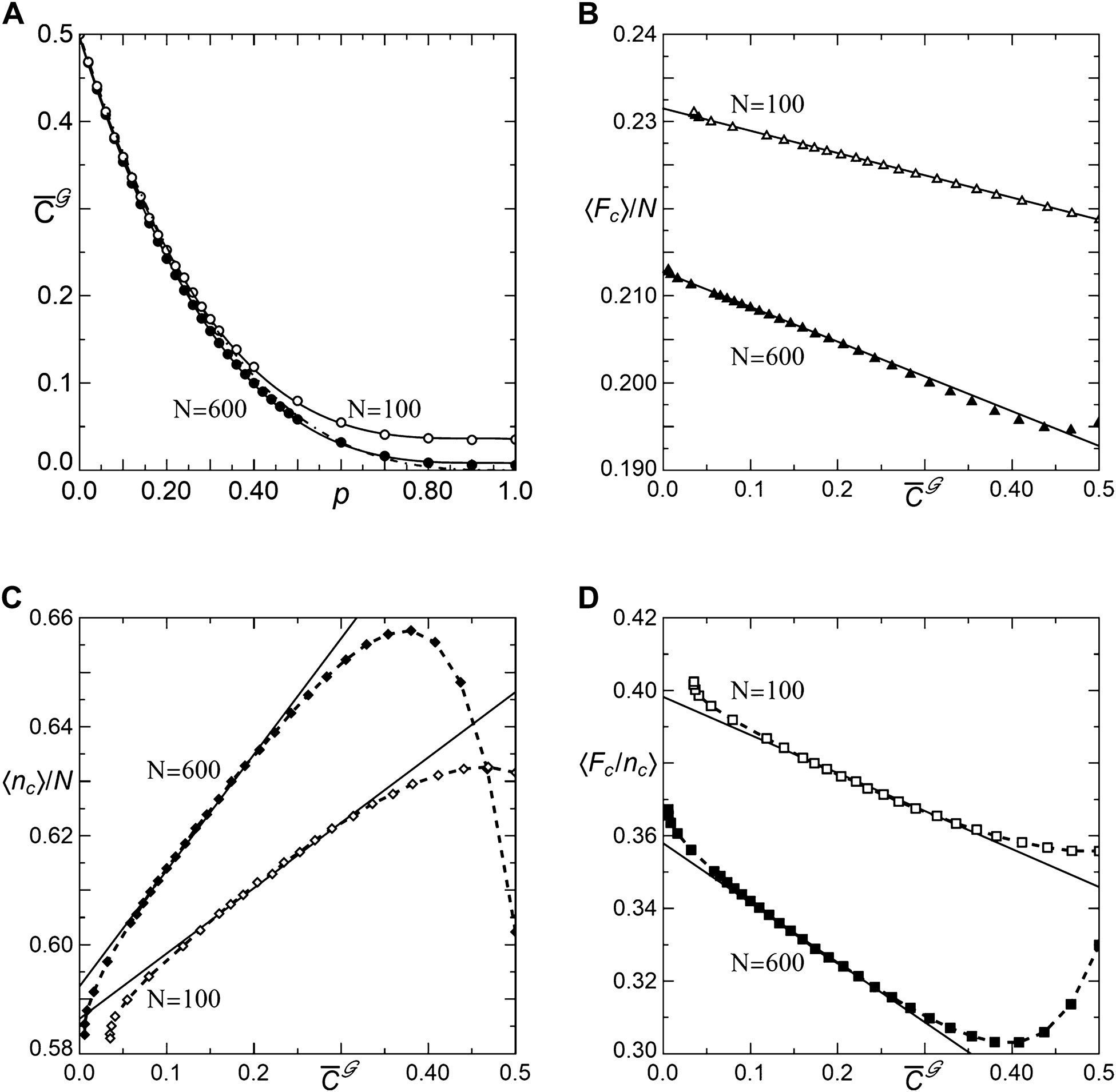
FIGURE 9. (A) Calculated mean empirical global clustering coefficient ${\overline{C}}^{\mathcal{G}}$ as a function of p for employed sets of 400 Watts-Strogatz graphs, each with connectivity $k=4$. The solid line is given by Eq. 9 with: $u=0.0358\pm 0.0004,w=0.4605\pm 0.0008,\xi =1.1\pm 0.007$, for $N=100$ and $u=0.0085\pm 0.0017,w=0.488\pm 0.001,\xi =1.076\pm 0.001$ for $N=600$). The dash-dotted line represents $C_{\infty }\left(p\right)=C\left(0\right){\left(1-p\right)}^3$, valid in the limit $N\to \infty$, where $C\left(0\right)=\left(3/4\right)\left(k-2\right)/\left(k-1\right)$ [37]. The diagrams (B–D) refer to: $\langle F_c/N\rangle$, $\langle n_c/N\rangle$, and $\langle F_c/n_c\rangle$, respectively on a linear scale for the ${\overline{C}}^{\mathcal{G}}$. Straight lines represent Eq. 10 and are drawn in accordance with parameters presented in Table 2. The dashed lines are visual guides. The sample size is equal to ${10}^6$ for each data point. Load thresholds are distributed uniformly.

TABLE 2

TABLE 2. Estimated coefficients in Eq. 10: $\langle Y\rangle =a_N+b_N\cdot {\overline{C}}_N^{\mathcal{G}}$, $N=100$ and 600, $\left\{\delta \right\}$: distributed uniformly over $\left(\mathrm{0,1}\right)$.

FIGURE 10

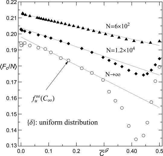
FIGURE 10. Mean strength of the system vs. mean global clustering coefficient for growing number of units. The linear scaling (11) between the ultimate strength $f_c^{\infty }$ and $C_{\infty }=\frac{1}{2}\left(1-p^3\right)$ is clearly seen.

When sets ${\left\{\delta \right\}}_{\mathcal{G}}$ are drawn from the Weibull distribution the relations (9) and (10) are present in systems with $N\sim {10}^2$, see Figure 11. When $\rho 5$ the relation (10) disappears gradually with an increase in N, as it is shown in Figure 12. This indicates that when ρ grows an ascending degree of order among load thresholds homogenizes the system and suppresses the linear relation between network’s clustering and system’s strength.

FIGURE 11

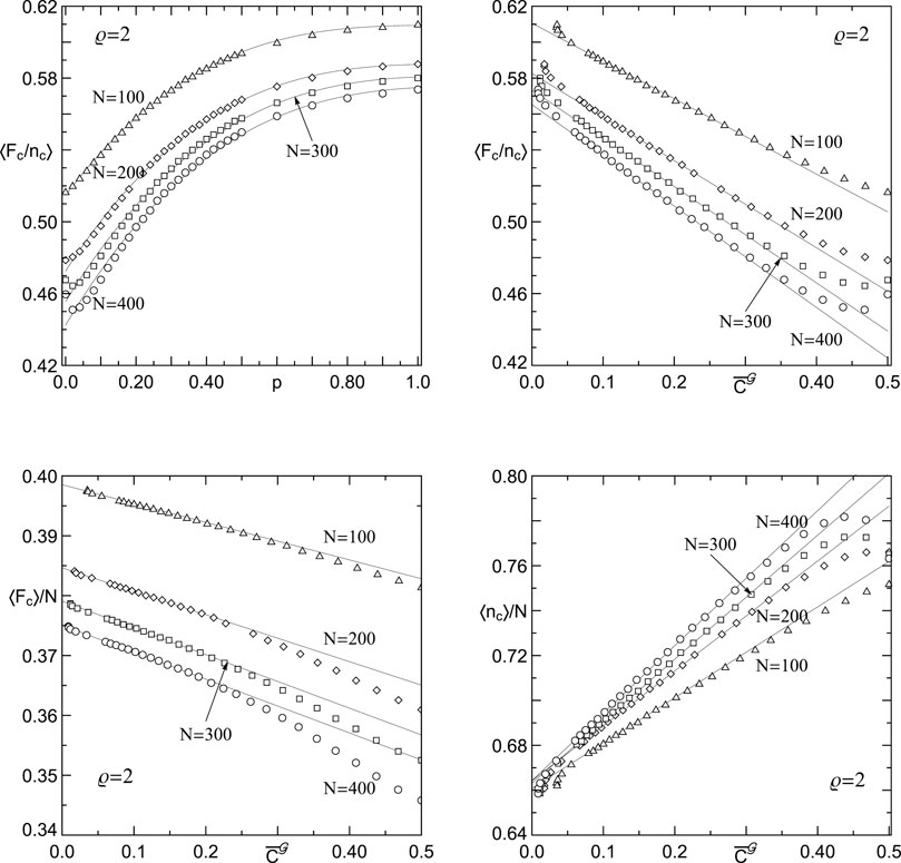
FIGURE 11. Upper panels: Mean system’s strength per reliable unit at critical configuration: (left) as function of p with solid lines drawn according to 9 and (right) on a linear scale for the respective mean ${\overline{C}}^{\mathcal{G}}$. Bottom panels: Mean system’s strength and mean number of reliable units at critical configuration, scaled by systems size N, as functions of mean empirical clustering coefficient calculated for corresponding networks. Results were obtained from ${10}^6$ samples with the Weibull distribution of $\left\{\delta \right\}$ for each data point.

FIGURE 12

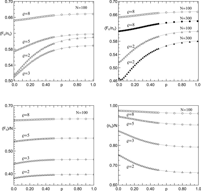
FIGURE 12. Scaled mean critical quantities: $\langle F_c/n_c\rangle ,\langle F_c\rangle /N$ and $\langle n_c\rangle /N$ for different values of Weibull shape parameter ρ and system size N as functions of p. The solid lines represent Eq. 9 with coefficients estimated from data. The sample size equals ${10}^6$.

It should be noticed that the expressibility of $\langle \cdot \rangle$ in ${\overline{C}}^{\mathcal{G}}\left(N,p\right)$ is not due to a kind of approximation or simplification that come from beyond the model but reflects a role that the small world structure of networks plays in maintaining functionalities of systems with strong to moderate load-threshold-disorder. It is also worth mentioning that the presented scaling results from: (i) the sLSG rule that allocates loads and (ii) the quasi-static method of load’s growth. It remains to be verified whether the scaling (10) is valid for other loading schemes.

Summary

We have investigated the evolution of failure among units that live at nodes of “small-world” networks and are exposed to a growing load. By introducing the sLGS rule of load transfer, which switches between the LLS and GLS rules depending on the accessibility of local interdependent nodes, we were able to mimic unit failures, and thus follow the evolution of the system toward the limit of its functionality. In particular, by employing the Watts-Strogatz random graphs to simulate the networks, we have collected data sufficient to form empirical distributions of the maximal load $F_c$, that would be safely supported by the minimal number $n_c$ of reliable units. These quantities have turned out to be skewed and adequately fitted by appropriate skew-normal distributions. The obtained distributions reflect: i) how $F_c,n_c$ and $F_c/n_c$ depend on number of units, and ii) how strongly they are affected by an amount of a network’s disorder, which is controlled by the rewiring probability p with which the links among interdependent nodes are modified.

The simulations show that if p is within the range of values given in Table 2 then $\langle F_c\rangle ,\langle n_c\rangle$ and $\langle F_c/n_c\rangle$ are linearly related to the global clustering coefficient averaged over the set of employed graphs. It should be noted, however, that even though our model sits on the Watts-Strogatz “small-world” networks, the obtained results are insensitive to the mean shortest path between pairs of nodes. This due to the sLGS rule that engages either the nearest-neighbouring nodes of a given node or all the other ones. Therefore, no distribution of distances appears in the presented results.

We are conscious of the fact that our simplified model of failure evolution involves some less realistic assumptions. Among the most serious is that we have considered each link between a pair of units as a reciprocally profitable relation. The other less strict assumption is that we allow the load thresholds be identically distributed. Our model can be tailored to fit a particular realistic scenario, e.g., by employing directed graphs, we would prevent some less reliable units from being interdependent.

Data Availability Statement

The raw data supporting the conclusions of this article will be made available by the author, without undue reservation.

Author Contributions

ZD performed the research and wrote the manuscript.

Conflict of Interest

The author declares that the research was conducted in the absence of any commercial or financial relationships that could be construed as a potential conflict of interest.

References

1. Lorenz J, Battiston S, Schweitzer F. Systemic risk in a unifying framework for cascading processes on networks. Eur Phys J B (2009) 71:441. doi:10.1140/epjb/e2009-00347-4

CrossRef Full Text | Google Scholar

2. Capelli A, Reiweger I, Lehmann P, Schweizer J. Fiber-bundle model with time-dependent healing mechanisms to simulate progressive failure of snow. Phys Rev E (2018) 98:023002. doi:10.1103/PhysRevE.98.023002

CrossRef Full Text | Google Scholar

3. Domanski Z. Damage statistics in progressively compressed arrays of nano-pillars. Eng Lett (2019a) 27:18–23.

Google Scholar

4. Hemmer PC, Pradhan S. Failure avalanches in fiber bundles for discrete load increase. Phys Rev E (2007) 75:046101. doi:10.1103/PhysRevE.75.046101

CrossRef Full Text | Google Scholar

5. Kim D-H, Kim BJ, Jeong H. Universality class of the fiber bundle model on complex networks. Phys Rev Lett (2005) 94:025501. doi:10.1103/PhysRevLett.94.025501

CrossRef Full Text | Google Scholar

6. Kun F, Raischel F, Hidalgo R, Herrmann H. Extensions of fibre bundle models. In: P Bhattacharyya BK Chakrabarti, editors Modelling critical and catastrophic phenomena in geoscience. Berlin, Heidelberg: Springer (2006) p 57–92.

Google Scholar

7. Pradhan S, Hansen A, Chakrabarti BK. Failure processes in elastic fiber bundles. Rev Mod Phys (2010) 82:499–555. doi:10.1103/RevModPhys.82.499

CrossRef Full Text | Google Scholar

8. Pugno NM, Bosia F, Abdalrahman T. Hierarchical fiber bundle model to investigate the complex architectures of biological materials. Phys Rev E (2012) 85:011903. doi:10.1103/PhysRevE.85.011903

CrossRef Full Text | Google Scholar

9. Hidalgo RC, Zapperi S, Herrmann HJ. Discrete fracture model with anisotropic load sharing. J Stat Mech Theor Exp (2008b) 2008:P01004. doi:10.1088/1742-5468/2008/01/P01004

CrossRef Full Text | Google Scholar

10. Hidalgo RC, Kovács K, Pagonabarraga I, Kun F. Universality class of fiber bundles with strong heterogeneities. EPL (2008a) 81:54005. doi:10.1209/0295-5075/81/54005

CrossRef Full Text | Google Scholar

11. Sbiaai H, Hader A, Boufass S, Achik I, Bakir R, Boughaleb Y. The effect of the substitution on the failure process in heterogeneous materials: fiber bundle model study. Eur Phys J Plus (2019) 134:148. doi:10.1140/epjp/i2019-12475-7

CrossRef Full Text | Google Scholar

12. Wang D, Jiang C, Park C. Reliability analysis of load-sharing systems with memory. Lifetime Data Anal (2017) 25:341–60. doi:10.1007s10985-018-9425-8

CrossRef Full Text | Google Scholar

13. Zhao X, Liu B, Liu Y. Reliability modeling and analysis of load-sharing systems with continuously degrading components. IEEE Trans Reliab (2018) 67:1096–110. doi:10.1109/TR.2018.2846649

CrossRef Full Text | Google Scholar

14. Hansen A, Hemmer P, Pradhan S. The fiber bundle model: modeling failure in materials. Weinheim, Germany: Viley-VCH (2015)

Google Scholar

15. Watts D, Strogatz S. Collective dynamics of ‘small-world’ networks. Nature (1998) 393:440–2. doi:10.1038/30918

CrossRef Full Text | Google Scholar

16. Jackson MO. An overview of social networks and economic applications. In: Benhabib J, Bisin A, Jackson M, editors. Handbook of social economics. Vol. 1A. North Holland, Netherlands: Elsevier (2012) p. 511–85.

Google Scholar

17. Newman M. The structure and function of complex networks. SIAM Rev (2003) 45:167–256. doi:10.1137/S003614450342480

CrossRef Full Text | Google Scholar

18. Burkholz R, Schweitzer F. Framework for cascade size calculations on random networks. Phys Rev E (2018) 97:042312. doi:10.1103/PhysRevE.97.042312

CrossRef Full Text | Google Scholar

19. Pradhan S, Chakrabarti BK, Hansen A. Crossover behavior in a mixed-mode fiber bundle model. Phys Rev E (2005) 71:036149. doi:10.1103/PhysRevE.71.036149

CrossRef Full Text | Google Scholar

20. Biswas S, Chakrabarti BK. Crossover behaviors in one and two dimensional heterogeneous load sharing fiber bundle models. Eur Phys J B (2013) 86:160. doi:10.1140/epjb/e2013-40017-4

CrossRef Full Text | Google Scholar

21. Kim BJ. Phase transition in the modified fiber bundle model. Europhys Lett (2004) 66:819–25. doi:10.1209/epl/i2004-10038-4

CrossRef Full Text | Google Scholar

22. La Rocca CE, Stanley HE, Braunstein LA. Strategy for stopping failure cascades in interdependent networks. Phys Stat Mech Appl (2018) 508:577–83. doi:10.1016/j.physa.2018.05.154

CrossRef Full Text | Google Scholar

23. Domanski Z. Statistics of flow through a multichannel supply system with random channel capacitances. IAENG J Appl Math (2019b) 43:18–23.

Google Scholar

24. Allen F, Gale D. Financial contagion. J Polit Econ (2000) 108:1–33. doi:10.1086/262109

CrossRef Full Text | Google Scholar

25. Boss M, Elsinger H, Summer M, Thurner S. Network topology of the interbank market. Quant Finance (2004) 4, 677–84. doi:10.1080/14697680400020325

CrossRef Full Text | Google Scholar

26. Cuadra L, Salcedo-Sanz S, Del Ser J, Jiménez-Fernández S, Geem Z. A critical review of robustness in power grids using complex networks concepts. Energies (2015) 8:9211–65. doi:10.3390/en8099211

CrossRef Full Text | Google Scholar

27. Pagani GA, Aiello M. The power grid as a complex network: a survey. Phys Stat Mech Appl (2013) 392:2688–700. doi:10.1016/j.physa.2013.01.023

CrossRef Full Text | Google Scholar

28. Rosas-Casals M, Valverde S, Solé RV. Topological vulnerability of the european power grid under errors and attacks. Int J Bifurc Chaos (2007) 17:2465–75. doi:10.1142/S0218127407018531

CrossRef Full Text | Google Scholar

29. Pagani GA, Aiello M. Towards decentralization: a topological investigation of the medium and low voltage grids. IEEE Trans Smart Grid (2011) 2:538–47. doi:10.1109/TSG.2011.2147810

CrossRef Full Text | Google Scholar

30. Saniee Monfared MA, Jalili M, Alipour Z. Topology and vulnerability of the iranian power grid. Phys Stat Mech Appl (2014) 406:24–33. doi:10.1016/j.physa.2014.03.031

CrossRef Full Text | Google Scholar

31. Cuadra L, Pino M, Nieto-Borge J, Salcedo-Sanz S. Optimizing the structure of distribution smart grids with renewable generation against abnormal conditions: a complex networks approach with evolutionary algorithms. Energies (2017) 10:1097. doi:10.3390/en10081097

CrossRef Full Text | Google Scholar

32. Sun Y, Tang X, Zhang G, Miao F, Wang P. Dynamic power flow cascading failure analysis of wind power integration with complex network theory. Energies (2017) 11:63. doi:10.3390/en11010063

CrossRef Full Text | Google Scholar

33. Zhang Z-Z, Xu W-J, Zeng S-Y, Lin J-R. An effective method to improve the robustness of small-world networks under attack. Chin Phys B (2014) 23:088902. doi:10.1088/1674-1056/23/8/088902

CrossRef Full Text | Google Scholar

34. Azzalini A. The skew-normal and related families. Cambridge, UK: Institute of Mathematical Statistics Monographs (Cambridge University Press) (2013)

Google Scholar

35. Arnold T, Emerson J. Nonparametric goodness-of-fit tests for discrete null distributions. R J (2011) 3:34–9. doi:10.32614/RJ-2011-016

CrossRef Full Text | Google Scholar

36. Wasserman L, Ramdas A, Balakrishnan S. Universal inference. Proc Natl Acad Sci USA (2020) 117:16880–90. doi:10.1073/pnas.1922664117

CrossRef Full Text | Google Scholar

37. Barrat A, Weigt M. On the properties of small-world network models. Eur Phys J B (2000) 13:547–60. doi:10.1007/s100510050067

CrossRef Full Text | Google Scholar