 Xiaojuan Tang
 Huiqiong Duan2
- 1School of Education, Jiangxi Normal University, Nanchang, China
- 2School of Foreign Languages, Nanchang Hangkong University, Nanchang, China
- 3School of Computer and Information Engineering, Jiangxi Normal University, Nanchang, China
- 4School of Public Administration, Nanchang University, Nanchang, China
Cognitive diagnostic test design (CDTD) has a direct impact on the pattern match ratio (PMR) of the classification of examinees. It is more helpful to know the quality of a test during the stage of the test design than after the examination is taken. The theoretical construct validity (TCV) is an index of the test quality that can be calculated without testing, and the relationship between the PMR and the TCV will be revealed. The TCV captures the three aspects of the appeal of the test design as follows: (1) the TCV is a measure of test construct validity, and this index will navigate the processes of item construction and test design toward achieving the goal of measuring the intended objectives, (2) it is the upper bound of the PMR of the knowledge states of examinees, so it can predict the PMR, and (3) it can detect the defects of test design, revise the test in time, improve the efficiency of test design, and save the cost of test design. Furthermore, the TCV is related to the distribution of knowledge states and item categories and has nothing to do with the number of items.
Introduction
Cognitive diagnosis (CD) has received much attention, providing diagnostic information of knowledge or skills (often called “attributes” in the CD literature) to the examinees (de la Torre and Douglas, 2004; de la Torre, 2008; DeCarlo, 2011; Liu et al., 2012; Kang et al., 2017; Huebner et al., 2018). It is critical to ensure that high-quality cognitive diagnostic tests can accurately diagnose the knowledge state (KS, i.e., the latent cognitive states) of examinees. The set of KSs is represented by the QS matrix. In fact, cognitive diagnostic test design (CDTD) is the design of a Q matrix, called Qt, i.e., rows representing attributes and columns representing attribute vectors, namely, items. By anchoring the items with attribute vectors, proposition experts and measurement experts transform items into measurable forms and then diagnose examinees. In a word, the design of the Qt matrix is the problem of how to match the attribute vectors to achieve a certain predetermined goal.
The CDTDs can be divided into the following aspects based on different dimensions: the dichotomous CDTD (Chiu et al., 2009; Ding et al., 2010) and the polytomous CDTD (Ding et al., 2014a,b,c) according to the scoring methods; Boolean matrix CDTD (Samejima, 1995; Tatsuoka, 1995, 2009; Ding et al., 2011; Cai et al., 2018) and polytomous Q matrix CDTD (Ding et al., 2015; Tu and Cai, 2015) according to the values of elements in the Qt matrix; model-dependent CDTD (Chiu et al., 2009; Kuo et al., 2016) and model-free CDTD (Shao, 2010) according to whether depending on the cognitive diagnostic models (CDM) or not; cognitive diagnostic computerized adaptive testing (CD-CAT) design (Cheng, 2010; Sun et al., 2019) and cognitive diagnostic testing (CDT) design (Henson and Douglas, 2005; Henson et al., 2008; Ding et al., 2011) according to whether personalized diagnostic; independent structure CDTD (Cheng, 2009, 2010; Liu et al., 2016) and dependent structure CDTD (Ding et al., 2011; Kuo et al., 2016) according to cognitive structure, and so on. In fact, almost all CDTDs are multidimensional.
Until present, the studies on the CDTD methods are still relatively weak, and they focus on the following two aspects:
(1) CDTD based on the perfect Q matrix
The so-called “perfect Q matrix” refers to the Qt matrix that makes the ideal response pattern (IRP) and KS correspond one to one. If the Q matrix in tests is a perfect Q matrix, the pattern match ratio (PMR) improves no matter whether the CDTD is either dichotomous or polytomous.
(i) Examples of dichotomous CDTD: For the four attribute hierarchies of Leighton (Leighton et al., 2004), if the Qt matrix is a Boolean matrix, and there is no compensation between the attributes, then the reachable matrix (or it is equivalent classes) acts as the submatrix of Qt which can achieve a one-to-one correspondence between the set of IRPs and the set of KSs. The more reachable matrices in the Qt matrix, the higher the PMR (Ding et al., 2010, 2011). Ding et al. (2010) called such a Qt matrix a sufficient and necessary matrix, i.e., a perfect Q matrix (Cai et al., 2018). The results are similar to those of Chiu et al. (2009), DeCarlo (2011), and Madison and Bradshaw (2015) on independent structures. With the independent structure and four attributes, Samejima (1995) believed that when the Qt matrix was the identity matrix (i.e., the identity matrix of independent structure is a reachable matrix), all of the KSs would not be misjudged. Chiu et al. (2009) also found that the Deterministic Input Noisy “AND” Gate (DINA) model and the Deterministic Input Noisy Output “OR” gate (DINO) model could diagnose all potential attribute mastery patterns when the Qt matrix included the identity matrix. Similar results have been addressed in other studies (DeCarlo, 2011; Madison and Bradshaw, 2015).
(ii) Examples of polytomous CDTD: To achieve the one-to-one correspondence between the set of KSs and the set of IRPs, the rooted tree structure, the independent structure, and the perfect Q matrices of the rhombus structure are introduced under the item score rule that one ideal score is added if mastering one attribute adhering to the item (Ding et al., 2014a). In the initial stage of CD-CAT, each attribute can be diagnosed by using the reachable matrix (Tu et al., 2013). In CD-CAT, the higher the percentage of the examinees is, whose testing items are (or contain) the reachable matrix according to the selection strategy, the higher the PRM is.
(2) CDTD based on the index
The Cognitive Diagnostic Index (CDI) (Henson and Douglas, 2005) and the Attribute-level Discrimination Index (ADI) (Henson et al., 2008) are based on the level of items and attributes for CD. Kuo et al. (2016) indicated that each attribute in the test must be measured at least three times to attain better correct attribute classification, so they proposed modified CDIs and ADIs, namely, MCDI and MADI. The Shannon's entropy (Xu et al., 2003) and posterior-weighted Kullback–Leibler (PWKL) (Cheng, 2009) were introduced in CD-CAT. Cheng (2010) believed that adequate coverage of each attribute could improve the validity of the test scores, and then the attribute-balancing index was proposed. Subsequently, the index was further improved (Yu et al., 2011; Liu et al., 2018; Sun et al., 2019). Adaptive multigroup testing method for cognitive diagnosis (CD-AMGT) (Luo et al., 2018), which selects a group of appropriate items in different diagnosis stages, has the advantages of uniform use of item bank and less time to calculate.
The PMR is the main evaluation index for cognitive diagnostic tests. In CDTD, the pretest evaluation of the PMR is more positive than the posttest evaluation because the designed test can be modified quickly, the designer can make up for possible errors before testing, and material resources and time will be saved. At present, the PMR is the posttest estimation based on the data measured or simulated, so it is impossible to calculate PMR immediately during the design process. Furthermore, it is meaningful to discuss the maximum PMR for the pretest, and the maximum PMR is related to the matching degree between the designed test and the cognitive model, as well as the quality and length of the test.
The rest of the study is organized as follows: First, the TCV used in this study is briefly described. Second, the theoretical proof of the relationships between the TCV and the PMR is introduced in detail. The TCV is then evaluated in a simulation study. The end of the study is the discussion and conclusion.
Methods
Cognitive Diagnosis
The cognitive model is a prerequisite for CD. It is represented by an attribute hierarchy, which specifies the psychological ordering of the attributes required to solve test items. Attributes are those basic cognitive processes or skills required to solve test items correctly. There are five forms of basic hierarchical structures (Leighton et al., 2004; Cheng, 2010), namely, A, B, C, D and E (Figure 1).
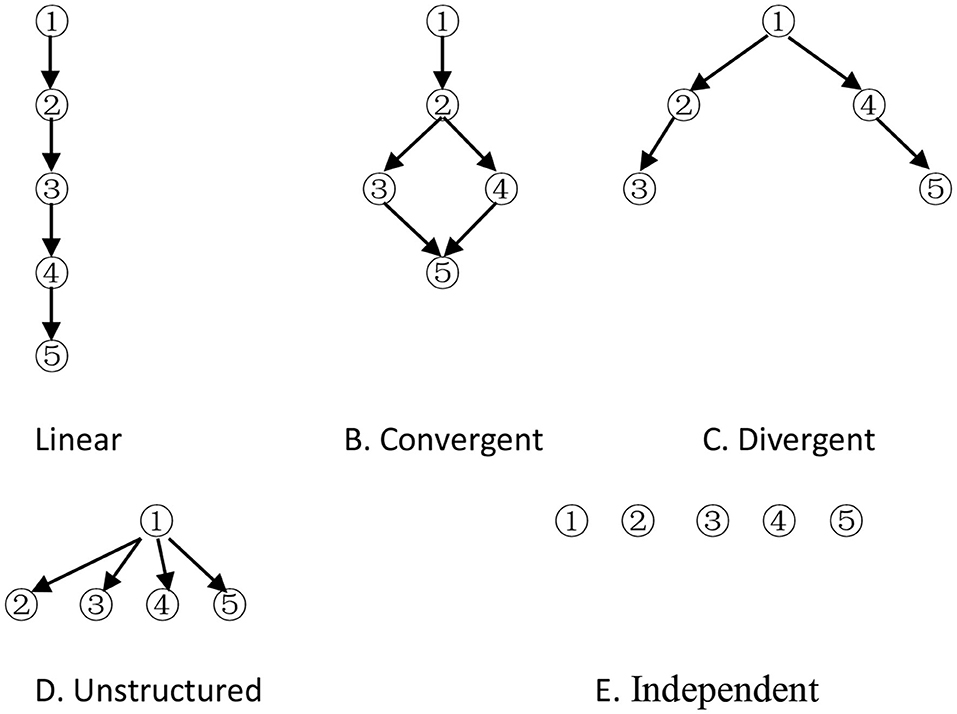
Figure 1. Five different hierarchical structures.
Attribute 1 is considered a prerequisite to other attributes, and attribute 5 depends on some attributes in models except the independent model. The adjacency (A), reachability (R), incidence (Q), and reduced incidence (Qr) matrices are specified by Tatsuoka (1995). The columns of the Qr matrix indicate that all possible items must be created to reflect the relationships among the attributes in the hierarchy. The possible latent cognitive states (i.e., KS), which is all the columns of the incidence matrix, possess cognitive attributes that are consistent with the hierarchy (when the hierarchy is based on cognitive considerations), and they apply these attributes systematically (when the hierarchy is based on procedural considerations) (Gierl et al., 2007). Let denote the jth dichotomous column vector (i.e., the jth category item) of the Qr matrix. All KSs are represented by column vectors: , where αik = 1(k = 1, ⋯ , K) indicates that the ith category examinee has mastered attribute k, and αik = 0 otherwise. K is the total number of attributes measured by the test. Let the Qs matrix denote all KSs, in fact, including zero vector ( i.e., this kind of examinee does not master any attribute) and the Qr matrix for cognitive attribute consistency. Thus, αi and qj are all K-dimensional vectors. The Qt matrix consists of some column vectors of the Qr matrix. Based on the cognitive model (including attributes and hierarchy among them), the Qr and Qs matrix can be obtained, that is, all possible items and KSs can be obtained. On the contrary, if the Qt matrix is known, some KSs can be obtained through the augment algorithm (Ding et al., 2008; Yang et al., 2008), and the cognitive model can be derived by comparing the rows (Tatsuoka, 1995). In general, it is impossible for some items (i.e., the Qt matrix) to replace all the items (i.e., the Qr matrix), which express the cognitive structure, so some cognitive structures extracted from the Qt matrix may be inconsistent with the theoretical one.
The DINA Model
Cognitive diagnostic models have been proposed for many years, including the rule space model (Tatsuoka, 1983), the “Noisy Input Deterministic ‘AND' Gate” (NIDA) model (Maris, 1999), the fusion model (Hartz, 2002), the reduced reparameterized unified model (R-RUM; Hartz, 2002), and the DINA model (Haertel, 1989). The DINA model is completely noncompensatory. The DINA model treats slipping and guessing at the item level. Parameter sj indicates the probability of “slipping,” and parameter gj denotes the probability of “guessing.” The item response function, therefore, can be written as follows:
When nij = 1, the ith examinee should be able to answer item j correctly, unless he/she “slips.” Similarly, when nij = 0, the ith examinee should not be able to answer item j correctly, unless he/she is a lucky guesser (Cheng, 2010).
Theoretical Construct Validity
Theoretical construct validity (TCV) is used to measure the degree of consistency between the theoretical cognitive model and the cognitive model implied in the Qt matrix (Ding et al., 2012).
Definition 1 Let {α1, α2, ⋯ , αN1} denote N1 KS of the theoretical cognitive model given by experts, {β1, β2, ⋯ , βN2} denote N2 KS derived from the Qt matrix, and {γ1, γ2, ⋯ , γN3} = {β1, β2, ⋯ , βN2}∩{α1, α2, ⋯ , αN1} denote N3 KS. when γk = αi, the TCV for the Qt matrix can be written as follows:
where pi represents the probability of the ith category examinees, that is, the ratio of such examinees whose KS is αi in the total population.
In particular, when all KS ratios in the total population are equal, then
In fact, the TCV is a measure of the degree to which the Qt matrix represents the theoretical cognitive model (Ding et al., 2012). The observed response pattern (ORP) and the CDM are necessary for the set of the estimation of KSs of the examinees. The set of IRPs is determined by the set of KSs, the test Q matrix, the element value of the Qt matrix (the dichotomous or the polytomous), the calculation method of the ideal score, the compensation between attributes, and so on. The ORP is related not only to the above mentioned factors but also to the item quality and random factors. Thus, if there is no random factor, the better the item quality, the closer the ORP is to the IRP. Due to the slipping and the guessing in the answering process of examinees, the PMR of the set of KSs estimated by the ORP is not higher than that estimated by the IRP, that is, PMRORP ≤ PMRIRP. The PMRIRP acts as the maximum PMRORP, and the smaller the slipping and the guessing, the more accurate the KSs based on the ORP. How to get the PMRIRP quickly is an interesting problem.
To clearly solve the interesting problem, a theoretical explanation that makes sense of the complexity is firmly couched within the examples.
Definition 2 Define the relationship between two attribute vectors αi and qj as αi ≥ qj if and only if αik ≥ qjk, for k = 1, 2, …, K. Strict inequality between the attribute vectors is involved (i.e., αi > qj) if αik > qjk for at least one k (de la Torre, 2011). αi ≤ qj and αi < qj can be defined similarly as mentioned earlier. If the relationship does not exist, then αi has nothing to do with qj. The definition of comparison between column vectors also applies to row vectors.
Examples
The theoretical cognitive model is an independent structure of three attributes, according to the methods suggested by Tatsuoka for calculating the adjacency (A), reachability (R), incidence (Q), and reduced incidence (Qr) matrices; then, adding zero vector to the Qr matrix, there are 23 = 8 possible KSs, that is, N1 is 8. The Qs matrix is represented by a 3 × 8 matrix as follows:
where αi (i = 1, ⋯ , 8) is the ith category examinees.
Test items, represented by a 3 × 3 matrix, can be written as follows:
where qj is the jth item when items are not duplicated, otherwise it represents the jth category item.
Calculation of TCV
A new matrix, called the is made of the Qt matrix and the two new columns. The two new columns based on the augment algorithm (Ding et al., 2008; Yang et al., 2008) are generated from the Qt matrix, while the non-zero vectors (0, 1, 1)T and (0, 0, 1)T in the Qs matrix cannot be generated as follows:
Five KSs in the are derived from the Qt matrix, that is, N2 is 5. There are five same possible latent cognitive states between the theoretical cognitive model and the cognitive model implied in the test design, that is, {γ1, γ2, γ3, γ4, γ5} = {α2, α3, α5, α6, α8}, N3 is 5 (N1, N2, and N3 are the same as Definition 1), when adding zero vector ().
(1) When the probability distribution of the set of KSs in the total population is discrete uniform, then TCV = (5 + 1)/8 = 3/4.
(2) Otherwise, suppose the ratios of all αi are 0.1, 0.1, 0, 1, 0.2, 0.1, 0.2, 0.1, 0.1, respectively, TCV = 0.1 + 0.1 + 0.1 + 0.2 + 0.1 = 0.6.
Calculation of PMRIRP
Ideal response (IR) depends on the relationship between αi and qj. Let denote that the ith examinee responses correctly on the jth item, and IR(αi, qj) = 0 otherwise. Clearly, IR(α1, q1) = IR(α1, q2) = IR(α1, q3) = 0 due to ; IR(α2, q1) = 1, IR(α2, q2) = IR(α2, q3) = 0 due to q1 ≤ α 2 < q3; and α 2 having nothing to do with q2. Similarly, the set of IRPs of the Qs matrix with respect to the Qt matrix is represented by a 3 × 8 matrix as follows:
In Equation 8, the row represents the item, and the column represents IRP. There are six different IRPs, that is, six KS can be correctly estimated without taking the slipping and the guessing into account. In essence, the estimated five KSs based on five IRPs are the same as vectors in the (five different categories), and adding estimated zero vector (because the IRP is zero vector), there are six categories. and are the same categories to zero vector () and , respectively; thus, no new categories are generated.
The whole process of dividing the Qs matrix can be vividly described as follows: the Qs matrix is similar to a line, and five vectors in the are similar to five dots that classify the line into six categories in which only one KS can be estimated correctly; therefore, .
From calculations 1 and 2, it can be known that TCV = PMRIRP.
Examples of other structures are shown in Table 1.
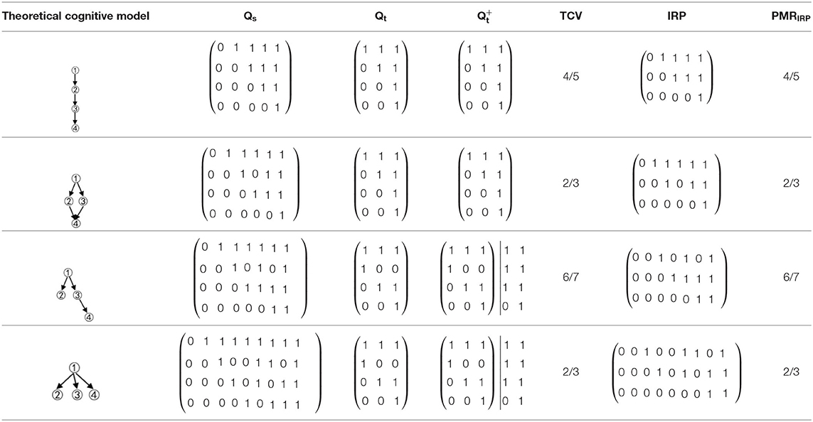
Table 1. The relationships between the theoretical construct validity (TCV) and the PMRIRP of other structures.
Although structures are different, convergent, or divergent, the result of the relationship between the TCV and the PMRIRP is the same: the number of vectors of the in the convergent structure was 3, and then the Qs matrix could be classified into four categories; the number of vectors of the in the divergent structure was 5 due to two new columns derived from the Qt matrix, and then the Qs matrix could be classified into six categories. For the linear structure and the unstructured, the results are similar.
Notably, all items of the Qt matrix are different because the repetition of items does not increase the “coverage” of the cognitive model by the Qt matrix. Repeated items only reduce random errors; thus, in the following discussion, it is not necessary to consider the repeated items in the Qt matrix.
Theoretical Derivation of TCV = PMRIRP
Let R denote reachable matrix, the Qr matrix is a set of all possible items that can be written as follows:
In fact, Qt ⊆ Qr, .
For every αi (i = 1, ⋯ , n) (except for zero vector) in the Qs matrix, there should be a corresponding to it, that is, α .
Based on the augment algorithm, the matrix can be defined as follows:
where V represents the Boolean union operation, p ∈ Q means that p is the item (column) of the Q matrix, and Q ⊆ Qt indicates that the Q matrix is a subset of the Qt matrix and contains one or more items. New columns of can be obtained by the Boolean union of two or more items in the Qt matrix. There are m columns in , adding zero vector, m+1 categories of the KSs are derived from the Qt matrix in total. n is the number of the set of KSs derived from the theoretical cognitive model, that is, n columns in the Qs matrix, so the TCV can be calculated as follows:
The maximum lower bound of αi can be found in by comparing αi with and it can be defined as follows:
In fact, j′ is the subscript of the maximum item, that is, , j′ ∈ {1, 2, ⋯ , m }.
Let denote a set of αi with the same maximum lower bound :
If does not exist, then let set as follows:
All the with the same IRP will be classified into one category by comparing αi with all p items in the Qt matrix: based on the definition of if exists, it means that , so the IRs between αi and p (p ≤ αi) are 1, that is, , the IRs between αi and the rest of p in the Qt matrix are 0, that is, IR (αi, p) = αip = 0. Therefore, all the in have the same IR, and these belong to one category. If does not exist, for all p items in the Qt matrix, αi < p or αi has nothing to do with p, the IRs between αi and p is 0, IR is the same with zero vector , and thus, these are the same category as zero vector.
Proposition 1: All αis in theQs matrix are classified into .
First, there must be existed a αi for every , so that αi, so is the maximum lower bound of αi, αi is an element of a m are divided into m sets .
Second, for the remaining n-m
(1) For every p in the Qt matrix, if αi < p or αi has nothing to do with p, then does not exist, so αi belongs to set ;
(2) If p ≤ αi, there must be existed acted as the maximum lower bound of αi, so αi belongs to set .
Combining (1) and (2), Proposition 1 is proved.
Proposition 2: If the number of qj in the matrix is m, all s in the Qs matrix are classified into m + 1 categories.
From Proposition 1, the conclusion is clearly true, that is, m + 1 categories of the set of KSs can be estimated correctly. Thus, . The result of TCV = PMRIRP shows that the TCV is equal to the PMR estimated by the set of IRPs. For PMRORP ≤ PMRIRP = TCV, the TCV is the upper bound of the PMR estimated by the ORP. When k is smaller, such as k ≤ 5, the TCV can be calculated by pen, otherwise, it is easily derived by using a computer.
Simulation Study
A simulation study was carried out to evaluate the relationships between the TCV and the PMR.
Five attribute hierarchical structures were studied, namely, independent, linear, convergent, divergent, and unstructured. The number of attributes was set at 4, that is, K = 4. The study needed to consider the influence of the distribution of examinees, item attribute vector, and their proportions on the TCV. Two kinds of distribution of the KSs of examinees were discussed as follows: the average distribution (30 persons for every KS) and the normal distribution. In particular, the standard multivariate normal distributions in the independent structure were investigated. The total number of examinees was the same. In contrast, there were six Qt matrices for each structure, items would be selected from the Qrmatrix, and its proportions were different. The test length was 20. The descriptive statistics of the examinees and the Qt matrices are reported in Table 2.
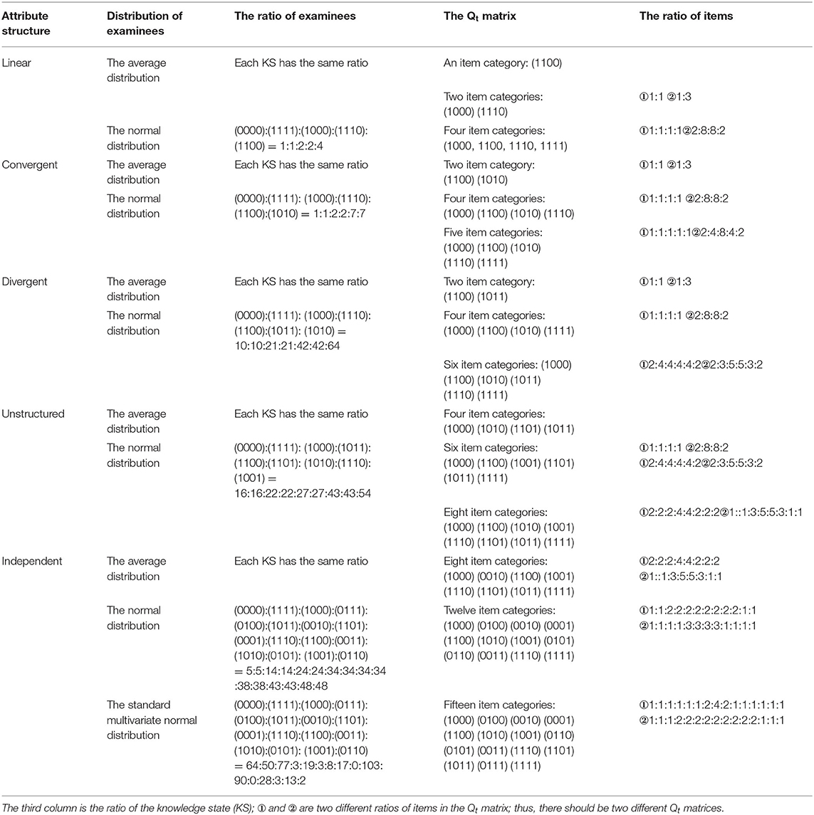
Table 2. The distributions of examinees and the proportions of items for five different hierarchical structures.
To compare the effects of different slips on the TCV and the PMR, the slips were 0.15 and 0.02, respectively. The set of IRPs was obtained by the items of the Qt matrix and the set of KSs of the Qs matrix. Let x denoted the IR score of an examinee on an item, r randomly generated from Uniform (0, 1), if r > 1 − s, x (x was dichotomous) would be changed to 1–x, and x otherwise.
The DINA model and the maximum-likelihood estimation method were used to estimate the KS. Considering the differences in the distribution of examinees, the Qt matrix, and the slips, there were 116 levels in total, and each level was tested 30 times. The final PRM was an average of 30 PMRs.
The PMR index can be defined as follows:
where N is the number of examinees. αi−correct = 1 represents that the ith examinee is estimated correctly.
Results
Table 3 compares the TCV and the PMR obtained from the linear structure. The first column shows the different distribution of examinees, and the other columns show the results of the different Qt matrices.
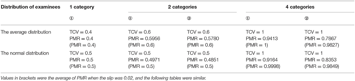
Table 3. The comparison between the TCV and the PMRORP of the linear structure.
Clearly, the TCV was superior: the TCV was uniformly higher than the PMR regardless of the distribution of examinees and the Qt matrices. Although the repetition of items in the Qt matrices, the TCV was not changed when the distribution of examinees and the category of items in the Qt matrices remain unchanged. Therefore, this helped in explaining why repeated items were not necessary to count. As is known to all, the smaller the slip is, the higher the PMR is. But the TCV had nothing to do with the slip, so the smaller the slip, the smaller the gap between the TCV and the PMR. For all the attribute structures, when the TCV was low, the PMR was also low and vice versa. Notably, the more the item categories were, the larger the TCV would be. In particular, if the Qt matrix contained the reachable matrix that could augment all possible item categories, then TCV = 1, regardless of the distribution of examinees. In other words, when the reachable matrix was a submatrix of the Qt matrix, the PMR would be higher than that of the Qt matrix that did not include the reachable matrix if the other conditions were the same.
From Tables 4–7, the data of other structures show the same results as linear. In addition, the lesser the structure, the greater the difference between the TCV and the PMR.
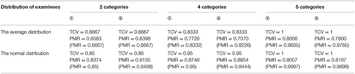
Table 4. The comparison between the TCV and the PMRORP of the convergent structure.
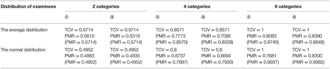
Table 5. The comparison between the TCV and the PMRORP of the divergent structure.
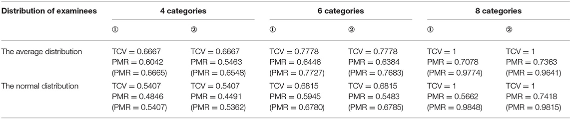
Table 6. The comparison between the TCV and the PMRORP of the unstructured structure.
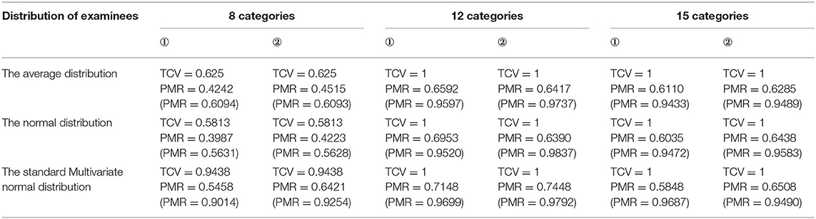
Table 7. The comparison between the TCV and the PMRORP of the independent structure.
Discussion and Conclusion
Guided by a cognitive model, the CD can detect how well the examinees have mastered certain knowledge or skills. All CDTDs aim at diagnosing examinees as much as possible, and the main evaluation index is the PMR. The higher the accuracy rate of the KSs, the higher the test construct validity. It is more meaningful to be able to calculate the PMR during CDTD. Tatsuoka (2009, p. 78–79) believed that the sufficient Q matrix can improve the test construct validity. However, how to measure the construct validity? Inspired by the evaluation of the sufficient Q matrix by Tatsuoka (1995, 2009), an evaluation index for cognitive diagnostic test (design) was developed, i.e., TCV, which made up for the defects of Tatsuoka's idea (Tatsuoka, 1995, 2009).
This study proposes a simplified method for predicting the PMR, namely, the TCV method for CD. The TCV intuitive meaning is as follows: the set of KSs is derived from the Qt matrix through the augment algorithm (i.e., this design can inspire some latent cognitive states), and if the probability distribution of the examinees in the population is known, then . In particular, when the probability distribution of the set of KSs in the total population is discrete uniform, the TCV is equal to the sum, which is the number of categories of the set of KSs derived from the Qt matrix plus 1, divided by the number of categories of the set of KSs in the population. In general, the TCV measures the degree of consistency between the cognitive model derived from matrix Qt and the theoretical cognitive model (Ding et al., 2012).
As the proof and the simulation showed, PMRORP ≤ PMRIRP = TCV. Therefore, the TCV can be used to predict the PMR. Notably, the TCV is related to the distribution of examinees and item category, not related to the proportion of items. In other words, when calculating the TCV, repeated items should be treated as one item.
The TCV is numerically equal to the PMR based on the set of IRPs, and the factors that affect the set of IRPs are as follows: the cognitive model (e.g., the number of attributes, attribute hierarchy, and compensation between attributes), the composition of the test matrix (e.g., Boolean matrix and multivalued Q matrix), the item score (e.g., 0–1 score or multilevel score). Whatever has an effect on the set of IRPs influences the TCV. When the test Q matrix (Qt) is a Boolean matrix, the score is 0 or 1, and the IR is 1 if and only if αi ≥ qj, the TCV is the upper bound of the PMR. The TCV has nothing to do with the CDM (i.e., classification method); therefore, the TCV is calculated by CDM-free. Thus, the conclusion is the same for the DINA model, the AHM (Attribute Hierarchy Method, Gierl et al., 2007) model, the RSM (Rule Space Method, Tatsuoka, 2009) model, and the GDD (Generalized Distance Discrimination, Sun et al., 2011) model.
The number of attributes has an effect on the TCV. For example, independent structure, if the probability distribution of the set of KSs in the total population is equal, different items containing only two attributes are selected, then when the number of attributes K is 3, and the TCV is 5/8; when K is 4, the TCV is 3/4; and when K is 5, the TCV is 27/32. However, under the same conditions, the number of attributes does not affect the conclusion that the TCV is the upper bound of the PMR at all (as shown by the proof). Furthermore, the lower the number of attributes, the higher the PMR. Therefore, the simulation study selected fewer attributes (K = 4). Similarly, the smaller the random in the ORP is, the higher the PMR is. To prove that the TCV is the upper bound of the PMR, in the simulation study, the random is relatively small (s = 0.02). According to the abovementioned logic, the result that TCV is the upper bound of the PMR is also true when the random is larger.
An interesting question arises as follows: the TCV is not equal to the PMR, why the TCV is useful for predicting the PMR? There are three reasons: First, the most important reason is that the TCV can be obtained during CDTD, which is instructive to adjust selected items at any time and to timely judge the test quality. Second, the TCV is the upper bound of the PMR, the smaller the slip, the smaller the gap between the TCV and the PMR. The TCV does not change with the slip. If the TCV is high, the PMR is also higher; therefore, it is feasible to use the TCV as an index of the PMR to predict the test quality. Third, the TCV is easy to calculate according to the formula.
The TCV can be used not only to predict the PMR but also, more importantly, to detect the defects of CDTD. By using the augment algorithm, the set of KSs can be derived from the Qt matrix, and then, the TCV can be calculated. Under the same conditions, if the TCV value is lower, it means that there are fewer kinds of attribute vectors (i.e., items) of the reachable matrix in the Qt matrix, and thus, the more KSs cannot be accurately estimated. At this time, test designers can modify the test Q matrix (i.e., the Qt matrix) before testing (not posttest evaluation), that is, modify the test (such as filling the columns of the reachable matrix or filling the columns expanded by the reachable matrix through the augment algorithm). Adjusting the selected items according to the TCV value at any time is not only beneficial to evaluate the test quality in time in CDTD but also can save cost and improve efficiency, which has the effect of two times the result with half the effort. This method undoubtedly has great advantages in CDTD.
If the test contains the reachable matrix, the cognitive model derived from the test is consistent with the theoretical cognitive model, and the TCV is 1. At this time, as long as the item quality is good (i.e., the slip is low) and attributes are measured a certain number of times, then the PMR is relatively high. In most cases, however, the PMR is not equal to 1 because the test is short, the quality of the items is poor, or the examinees do not answer carefully. At this time, although the result is rough when the TCV is used to predict the PMR, even so, under the same cases, the test, which contained the reachable matrix (in this case, the Qt matrix is complete Q matrix, Cai et al., 2018), has the higher PMR.
Although this study shows that the TCV method works successfully with CD, it has limitations in several aspects: (1) Since the TCV is determined by the Qt matrix, the Qt matrix must be complete and reliable, which is the premise of using the TCV. In some cases, this condition may be quite harsh. But the RUM model allows the Qt matrix to be incomplete, and the conclusion of this study cannot be applied. Furthermore, the complete and accurate calibration of the Qt matrix is still a very difficult problem. (2) If the score is 0 or 1 and IR is 1 if αi ≥ qj, other IR rules are not applicable in this case. Nor does it apply if there is compensation between attributes. (3) Only the dichotomous and non-compensable attributes are considered, a natural question that arises is how to get the TCV when the scoring is polytomous and attributes are compensable. These will be the interesting topics for future studies.
Data Availability Statement
The raw data supporting the conclusions of this article will be made available by the authors, without undue reservation.
Author Contributions
XT designed the study, conducted the simulation study, and wrote the manuscript. SD, HD, and MM revised the manuscript. All authors contributed to the article and approved the submitted version.
Funding
This research was partially supported by the National Natural Science Foundation of China (Grant No. 31360237, 31500909, 61967009, 62067005), the National Social Science Foundation of China (Grant No. 13BYY087), the Project of Teaching Reform of Jiangxi (Grant No. JXJG-19-2-16), the Project of Education Sciences Planning of Jiangxi (Grant No. 20YB028), the Project of Humanity and Social Science Youth Foundation of the Ministry of Education (Grant No. 16yjc190016), and the Project of Graduate Innovation Special Foundation of Jiangxi (Grant No. YC2019033).
Conflict of Interest
The authors declare that the research was conducted in the absence of any commercial or financial relationships that could be construed as a potential conflict of interest.
Publisher's Note
All claims expressed in this article are solely those of the authors and do not necessarily represent those of their affiliated organizations, or those of the publisher, the editors and the reviewers. Any product that may be evaluated in this article, or claim that may be made by its manufacturer, is not guaranteed or endorsed by the publisher.
References
Cai, Y., Tu, D., and Ding, S. (2018). Theorems and methods of a complete Q matrix with attribute hierarchies under restricted q-matrix design. Front. Psychol. 9:1413. doi: 10.3389/fpsyg.2018.01413
Cheng, Y. (2009). When cognitive diagnosis meets computerized adaptive testing: CD-CAT. Psychometrika 74, 619–632. doi: 10.1007/s11336-009-9123-2
Cheng, Y. (2010). Improving cognitive diagnostic computerized adaptive testing by balancing attribute coverage: the modified maximum global discrimination index method. Educ. Psychol. Measur. 70, 902–913. doi: 10.1177/0013164410366693
Chiu, C. Y., Douglas, J. A., and Li, X. D. (2009). Cluster analysis for cognitive diagnosis: theory and applications. Psychometrika 74, 633–665. doi: 10.1007/s11336-009-9125-0
de la Torre, J. (2008). An empirically based method of Q-matrix validation for the DINA model: development and applications. J. Educ. Measure. 45, 343–362. doi: 10.1111/j.1745-3984.2008.00069.x
de la Torre, J. (2011). The generalized DINA model framework. Psychometrika 76, 179–199. doi: 10.1007/s11336-011-9207-7
de la Torre, J., and Douglas, J. A. (2004). Higher-order latent trait models for cognitive diagnosis. Psychometrika 69, 333–353. doi: 10.1007/BF02295640
DeCarlo, L. T. (2011). On the analysis of fraction subtraction data: the DINA model, classification, latent class sizes, and the Q-matrix. Appl. Psychol. Measure. 35, 8–26. doi: 10.1177/0146621610377081
Ding, S. L., Luo, F., Cai, Y., Lin, J., and Wang, X. B. (2008). “Complement to Tatsuoka's Q matrix theory,” in New Trends in Psychometrics, eds K. shigemasu, A. Okada, T. Imaizumi, and T. Hoshino (Tokyo, Japan: Universal Academy Press, Inc.), 417–423.
Ding, S. L., Mao, M. M., Wang, W. Y., Luo, F., and Cui, Y. (2012). Evaluating the consistency of test items relative to the cognitive model for educational cognitive diagnosis. Acta Psychol. Sinica 44, 1535–1546. doi: 10.3724/SP.J.1041.2012.01535
Ding, S. L., Luo, F., and Wang, W. Y. (2014a). Design of polytomous cognitively diagnostic test blueprint-for the independent and the rhombus attribute hierarchies. J. Jiangxi Normal Univ. 38, 265–268. doi: 10.16357/j.cnki.issn1000-5862.2014.03.012
Ding, S. L., Luo, F., Wang, W. Y., and Xiong, J. H. (2014c). The designing cognitive diagnostic test with dichotomous scoring. J. Jiangxi Normal Univ. 43, 441–447. doi: 10.16357/j.cnki.issn1000-5862.2019.05.01
Ding, S. L., Wang, W. Y., and andYang, S. Q. (2011). The design of cognitive diagnostic test blueprints. J. Psychol. Sci. 34, 258–265.
Ding, S. L., Wang, W. Y., and Luo, F. (2014b). The word frequency effect of fovea and its effect on the preview effect of parafovea in Tibetan reading. J. Jiangxi Normal Univ. 38, 111–118.
Ding, S. L., Wang, W. Y., Luo, F., and Xiong, J. H. (2015). The polytomous Q- matrix theory. J. Jiangxi Normal Univ. 39, 365–370. doi: 10.16357/j.cnki.issn1000-5862.2015.04.07
Ding, S. L., Yang, S. Q., and Wang, W. Y. (2010). The importance of reachability matrix in constructing cognitively diagnostic testing. J. Jiangxi Normal Univ. 34, 490–494. doi: 10.16357/j.cnki.issn1000-5862.2010.05.023
Gierl, M. J., Leighton, J. P., and Hunka, S. M. (2007). “Using the attribute hierarchy method to make diagnostic inferences about examinees' cognitive skills,” in Cognitive Diagnostic Assessment for Education: Theory and Applications, eds J. P. Leighton and M. J. Gierl (New York, NY: Cambridge University Press), 242–274.
Haertel, E. H. (1989). Using restricted latent class models to map the skill structure of achievement items. J. Educ. Measure. 26, 333–352. doi: 10.1111/j.1745-3984.1989.tb00336.x
Hartz, S. (2002). A Bayesian Framework for the Unified Model for Assessing Cognitive Abilities: Blending Theory with Practicality, Unpublished doctoral dissertation University of Illinois at Urbana-Champaign: Champaign, IL.
Henson, R. A., and Douglas, J. (2005). Test construction for cognitive diagnostics. Appl. Psychol. Measure. 29, 262–277. doi: 10.1177/0146621604272623
Henson, R. A., Roussos, L., Douglas, J., and He, X. (2008). Cognitive diagnostic attribute-level discrimination indices. Appl. Psychol. Measure. 32, 275–288. doi: 10.1177/0146621607302478
Huebner, A., Finkelman, M. D., and Weissman, A. (2018). Factors affecting the classification accuracy and average length of a variable-length cognitive diagnostic computerized test. J. Comput. Adapt. Test. 6, 1–14. doi: 10.7333/1802-060101
Kang, H. A., Zhang, S. S., and Chang, H. H. (2017). Dual-objective item selection criteria in cognitive diagnostic computerized adaptive testing. J. Educ. Measure. 54, 165–183. doi: 10.1111/jedm.12139
Kuo, B. C., Pai, H. S., and de la Torre, J. (2016). Modified cognitive diagnostic index and modified attribute-level discrimination index for test construction. Appl. Psychol. Measure. 40, 315–330. doi: 10.1177/0146621616638643
Leighton, J. P., Gierl, M. J., and Hunka, S. M. (2004). The attribute hierarchy method for cognitive assessment: a variation on Tatsuoka's rule-space approach. J. Educ. Measure. 41, 205–237. doi: 10.1111/j.1745-3984.2004.tb01163.x
Liu, J. C., Xu, G. J., and Ying, Z. L. (2012). Data-driven learning of Q-matrix. Appl. Psychol. Measure. 36, 548–564. doi: 10.1177/0146621612456591
Liu, R., Huggins-Manley, A. C., and Bradshaw, L. (2016). The impact of Q-matrix designs on diagnostic classification accuracy in the presence of attribute hierarchies. Educ. Psychol. Measure. 77, 220–240. doi: 10.1177/0013164416645636
Liu, S. C., Tu, D. B., Cai, Y., and Zhao, Y. (2018). Four new item selection strategies based on attribute balancing in CD-CAT. Psychol. Sci. 41, 976–981. doi: 10.16719/j.cnki.1671-6981.20180432
Luo, F., Wang, X. Q., Ding, S. L., and Xiong, J. H. (2018). The design and selection strategies of adaptive multi-group testing for cognitive diagnosis. Psychol. Sci. 41, 720–726. doi: 10.16719/j.cnki.1671-6981.20180332
Madison, M. J., and Bradshaw, L. P. (2015). The effects of Q-matrix design on classification accuracy in the log-linear cognitive diagnosis model. Educ. Psychol. Measure. 75, 491–511. doi: 10.1177/0013164414539162
Maris, E. (1999). Estimating multiple classification latent class models. Psychometrika 64, 187–212. doi: 10.1007/BF02294535
Samejima, F. (1995). “A cognitive diagnosis method using latent trait models: competency space approach and it s relationship with DiBelloand Stout' s Unified Cognitive-Psychometric Diagnosis Model,” in Cognitively Diagnostic Assessment, eds P. D. Nichols, S. F. Chipman, and R. L. Brennan (Hillsdale, NJ: Erlbaum), 391–410.
Shao, H. (2010). Cognitive Diagnosis and its Application for the Surface Similarity Test of Children's Analogical Reasoning (Unpublished master's thesis). Jiang xi Normal University.
Sun, J. N., Zhang, S. M., Xin, T., and Bao, Y. (2011). A cognitive diagnosis method based on Q-Matrix and generalized distance. Acta Psychol. Sin. 43, 1095–1102. doi: 10.3724/SP.J.1041.2011.01095
Sun, X. J., Wang, Y. T., Zhang, S. Y., and Xin, T. (2019). New methods to balance attribute coverage for cognitive diagnostic computerized adaptive testing. Psychol. Sci. 42, 1236–1244. doi: 10.16719/j.cnki.1671-6981.20190531
Tatsuoka, K. K. (1983). Rule space: an approach for dealing with misconceptions based on item response theory. J. Educ. Measure. 20, 345–354. doi: 10.1111/j.1745-3984.1983.tb00212.x
Tatsuoka, K. K. (1995). “Architecture of knowledge structures and cognitive diagnosis: a statistical pattern classification approach,” in Cognitively Diagnostic Assessments, eds P. D. Nichols, S. F. Chipman, R. L. Brennan (Hillsdale, NJ: Erlbaum), 327–359.
Tatsuoka, K. K. (2009). Cognitive Assessment: An Introduction to the Rule Space Method. New York, NY: Taylor and Francis Group.
Tu, D. B., and Cai, Y. (2015). The development of CD-CAT with polytomous attributes. Acta Psychol. Sinica 47, 1405–1414. doi: 10.3724/SP.J.1041.2015.01405
Tu, D. B., Cai, Y., and Dai, H. Q. (2013). Item selection strategies and initial items selection methods of CD_CAT. J. Psychol. Sci. 36, 469–474. doi: 10.16719/j.cnki.1671-6981.2013.02.040
Xu, X., Chang, H., and Douglas, J. (2003). “Computerized adaptive testing strategies for cognitive diagnosis,” in Paper Presented at the Annual Meeting of National Council on Measurement in Education, Montreal, Canada.
Yang, S. Q., Cai, S. Z., Ding, S. L., Lin, H. J., and Ding, Q. L. (2008). Augment algorithm for reduced Q-matrix. J. Lanzhou Univ. 44, 87–91, 96. doi: 10.13885/j.issn.0455-2059.2008.03.027
Keywords: cognitive diagnostic test design, pattern match ratio, theoretical construct validity, prediction method, upper bound
Citation: Tang X, Duan H, Ding S and Mao M (2021) A Simplified Method for Predicting Pattern Match Ratio. Front. Psychol. 12:704724. doi: 10.3389/fpsyg.2021.704724
Received: 03 May 2021; Accepted: 26 July 2021;
Published: 03 September 2021.
Edited by:
Tao Xin, Beijing Normal University, ChinaReviewed by:
Ren Liu, University of California, Merced, United StatesChunhua Kang, Zhejiang Normal University, China
Copyright © 2021 Tang, Duan, Ding and Mao. This is an open-access article distributed under the terms of the Creative Commons Attribution License (CC BY). The use, distribution or reproduction in other forums is permitted, provided the original author(s) and the copyright owner(s) are credited and that the original publication in this journal is cited, in accordance with accepted academic practice. No use, distribution or reproduction is permitted which does not comply with these terms.
*Correspondence: Xiaojuan Tang, cHN5Y2hvdGFuZ0Bmb3htYWlsLmNvbQ==; Shuliang Ding, ZGluZzA2MDI2QDE2My5jb20=