Flow-State Identification of Oil-Based Magnetic Fluid Seal Based on Acoustic Emission Technology

Introduction

The magnetic fluid seal is a new seal technology controlled by a magnetic field. Magnetic fluid is injected in the gap of a magnetic circuit comprising a permanent magnet, pole shoes, and rotating shaft to form several magnetic fluid “O” rings. It has the advantages of zero leakage, long service life, and high reliability compared with other seal technologies. So, it has an important application value in aerospace, military, and other fields (Li and Hao, 2018). Its good seal performance is the premise for these fields’ normal functioning.

The pressure signal has often been used to characterize magnetic fluid seal performance at present. Chen (2019) judged each magnetic fluid “O” ring’ seal performance by the pressure signal of the cavity between the two pole shoes. Wang (2019) designed a new seal structure with two seal units. The pressure detection devices distributed between them can monitor magnetic fluid sealing liquid medium’s performance online and realize seal failure warning. The holes must be drilled on the seal element to connect the pressure detection devices. The more holes are drilled, the more leakage points exist, which is more unfavorable to the seal effect. According to the flow simulation model established by Chen (2019) when studying the mechanism of magnetic fluid seal, its seal performance is closely related to the flow state of magnetic fluid. When conducting experiments under static conditions, he unfolded the rotating structure along the circumference, pressed the front and rear end faces with transparent materials to achieve seal, and photographed magnetic fluid flow with a macro camera. Wang (2019) used a transparent shell, changed pole teeth’s location and shape to achieve seal, and captured the magnetic fluid’s interface changes with a camera. Kurfess and Müller (1990) transformed the rotating shaft into a hollow glass rod. The plane mirror extended into it and reflected the magnetic fluid’s flow change, which can be observed by a microscope. The way of camera shooting or microscope observation needs to change the seal structure and replace it with transparent materials, which is not universal.

The abovementioned research studies are all carried out on the experimental platform. In practical applications, magnetic fluids are mostly wrapped by opaque devices. They are not allowed to be disassembled at will after assembly. Therefore, new nondestructive testing technology is needed to monitor the flow state of magnetic fluid in the seal gap.

Liquid film seal is a non-contact mechanical seal based on the hydrodynamic lubrication theory. A micron groove with certain geometry is set on the end face of the seal ring. A full-liquid film is formed based on the dynamic pressure effect between end faces during the seal operation. Maintaining the liquid film’s stable existence is the key to ensuring good liquid film seal performance (Li, 2017).

Sun et al. (2018) pointed out that acoustic emission technology applied to liquid film seal monitoring is a new development direction in the seal field. The friction between the moving and stationary ring as a secondary sound source can be detected by an acoustic emission sensor. Relevant studies include the monitoring of the seal opening process and liquid film thickness (Li et al., 2014; Jiang, 2015; Zhang, 2015; Ge et al., 2016; Li, 2016; Zhang, 2016). Jiang (2015) distinguished the three friction states (dry friction, mixed friction, and fluid friction) in the seal opening process, then collected the acoustic emission signal and performed wavelet packet analysis, extracted time-frequency domain eigenvalues, and took them as input to train the Elman network model to identify the different friction states. Li (2016) pointed out that different film thicknesses will lead to different degrees of friction between dynamic and static rings, so the acoustic emission signal can be connected with the film thickness. Li et al. (2014) divided the film thickness into three states (thin, medium, and thick), found the corresponding acoustic emission signals and performed empirical mode decomposition (EMD), and then proposed a dual back propagation (BP) neural network to identify the different states. In a word, most of the current research studies collect the acoustic emission signals as samples and use machine learning methods to identify different states of the liquid film seal.

In the process of magnetic fluid flow, there is viscous friction of fluid and friction between the fluid and solid walls such as rotating shaft and pole shoes. Therefore, acoustic emission technology is used to monitor the flow state of the oil-based magnetic fluid in the seal gap in this study based on the similarity between the magnetic fluid seal and liquid film seal. The time- and frequency-domain features are extracted from the acoustic emission signal samples, and the random forest model based on the grey wolf optimizer is trained to identify the different states before seal failure. The effectiveness of this monitoring method is verified by the results.

Collection of Acoustic Emission Signal Samples

In order to explore the information of the oil-based magnetic fluid flow for rotating shaft seals, an experiment of sealing gas with oil-based magnetic fluid under static conditions is designed. The acoustic emission and pressure signals are collected at the same time in this experiment. With the aid of pressure signals, the acoustic emission signal samples of different states are collected.

Introduction of the Experiment Devices

The experimental devices include an acoustic emission sensor, 2/4/6 preamplifier, pressure transmitter, data acquisition instrument, 24 V DC power supply, air compressor, pressure relief valve, and so on. The connection diagram of these devices is shown in Figure 1.

FIGURE 1

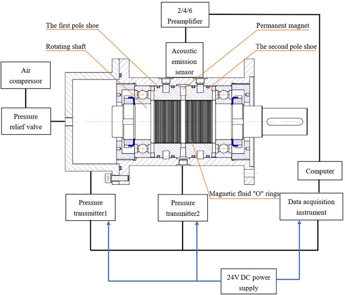
FIGURE 1. Connection diagram of the experimental devices.

The rotating shaft seal element has two-stage pole shoes. The oil-based magnetic fluid’s theoretical maximum pressure is 323.08 kPa under static conditions. The propagation distance is an important factor affecting the attenuation degree of the acoustic emission signal. The distance from the magnetic fluid to shell is about 25 mm in this structure. The cylindrical magnets are arranged closely along the circumference to provide a magnetic field, and there is a gap between the two adjacent cylindrical magnets. Therefore, the pressure transmitter 2 can detect the gas leaked after the first-stage pole shoe (close to the seal cavity) seal failure, and the pressure measured reflects the first-stage seal state. The oil-based magnetic fluid seal state of the two-stage pole shoe is reflected by pressure transmitter 1. The cycle of pressure data acquisition is 0.04 s. The PICO acoustic emission sensor produced by the American Physical Acoustics Company (PAC) is used for acoustic emission signal acquisition. A coupling agent is coated on the contact between the sensor and shell to reduce signal loss and fix the acoustic emission sensor between the two pole shoes with transparent glue. Acoustic emission signals are collected and stored by AE-win software after being amplified by a 2/4/6 preamplifier. The software can record a short-time acoustic emission wave at regular cycles with a specified sampling rate and a specified number of sampling points. The data contained in each short-time wave can be saved as a text document, and each text document will be regarded as a sample for subsequent state recognition research. As shown in Figure 2, the recording cycle of the short-time wave is set as $T_w=1.3\mathrm{ms}$, the sampling rate is $f_s=2\text{MHz}$, and sampling points $N=1024$.

FIGURE 2

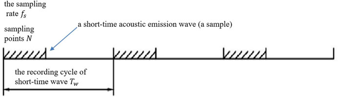
FIGURE 2. Schematic diagram of the acoustic emission signal acquisition mode.

Process of the Experiment

1) Clean the disassembled parts with kerosene and then make them dry. Inject $1\text{mL}$ oil-based magnetic fluid into the pole shoes. Reassemble the seal devices and rotate the rotating shaft to make oil-based magnetic fluid distribution more uniform.

2) Connect the pipeline and paste the sensor as shown in Figure 1.

3) Turn on the power supply and inflate the air pump of the air compressor to 700 kPa (greater than the theoretical maximum pressure of the seal element).

4) Click the acoustic emission and pressure signal acquisition software at the same time to start data acquisition. Start the air pump. Adjust the pressure relief valve knob clockwise manually and pressurize slowly until the seal fails.

5) Adjust the knob counterclockwise to close the pressure relief valve and stop inflation. Stop collecting the signals and save the data.

6) Turn off the power and disassemble devices. Adjust the pressure relief valve knob clockwise to discharge the remaining gas in the air pump.

7) Disassemble the seal element and clean it for the next experiment.

Analysis of Experiment Results

The pressure variation is shown in Figure 3. Phase I does not supply air to the seal cavity, and there is no magnetic fluid flow in this time period. Therefore, there is only noise signal. Phase II begins to pressurize the seal cavity. When the pressure of the seal cavity is greater than the first pole tooth magnetic fluid’s maximum pressure, the magnetic fluid begins to flow. Therefore, there is only noise signal in the front part of this phase, and the latter part is the mixture of noise and the first pole shoe magnetic fluid flow signals. But, the exact time of magnetic fluid beginning to flow cannot be judged only by the pressure curve. The stepped pressure rise in phase III represents the first pole shoe seal failure. Then, it basically remains horizontal, indicating the first pole shoe magnetic fluid has a self-healing phenomenon and plays a seal role again. The horizontal section has a slightly inclined downward trend and fluctuation phenomenon, which indicates the second pole shoe magnetic fluid flows. The pressure of both transmitters drops in phase Ⅳ, which represents two-stage pole shoe seal failure.

FIGURE 3

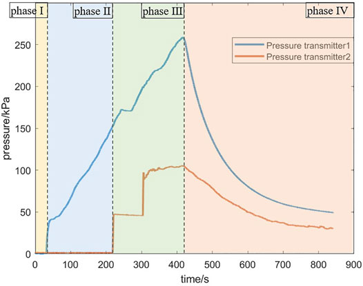
FIGURE 3. Pressure variation in the oil-based magnetic fluid seal experiment.

Next, the acoustic emission signal is analyzed. The directly collected acoustic emission data often has a lot of noise interference, which is reflected in the curve by some “burrs and spikes”. If the noise is too large, the useful information will be covered up. So, we use the “moving average of (2n + 1) points” in MATLAB to smooth and preprocess original data. The principle is to take out $2n+1$ data $\left(y_{i-n}, \dots ,y_{i-1},y_i, y_{i+1}, \dots ,y_{i+n}\right)$ that centered on $y_i$. Also, their average is calculated to replace $y_i$. Namely,

$y_i^{\prime }=\frac{1}{2n+1}{\displaystyle \sum _{k=-n}^n{y}_{i+k}},(1)$

where $y_{i+k}$ is the original data and $y_i^{\prime }$ is the smoothed data. In this study, n = 25. The time-domain diagram of the acoustic emission signal is shown in Figure 4. The smoothed curve can reflect the overall trend of continuous signal change.

FIGURE 4

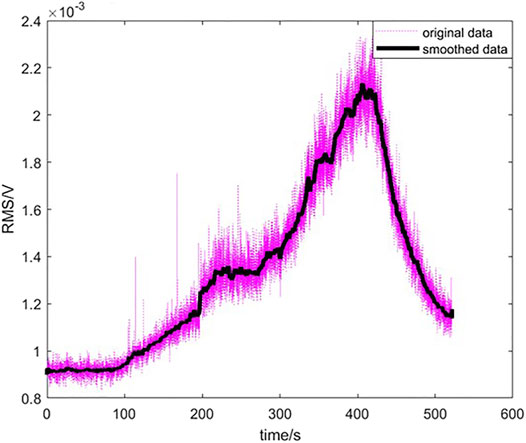
FIGURE 4. Time-domain curve of the acoustic emission signal in the experiment.

Segment the smoothed acoustic emission signal with the aid of the pressure signal at the same time point. As shown in Figure 5, the acoustic emission signal in phase I is constant, indicating stable noise interference in this experiment. The rising acoustic emission signal in phases II and III contains the information on oil-based magnetic fluid flow. In phase Ⅳ, the acoustic emission signal decreases after complete leakage, which means the magnetic fluid flow becomes weaker and weaker.

FIGURE 5

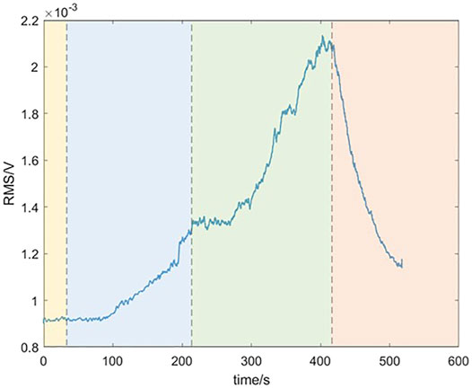
FIGURE 5. Smoothed acoustic emission signal segmentation in the experiment.

Select different pressure points at each phase, as shown in Figure 6, and analyze the power spectrum of the acoustic emission signal at that time.

FIGURE 6

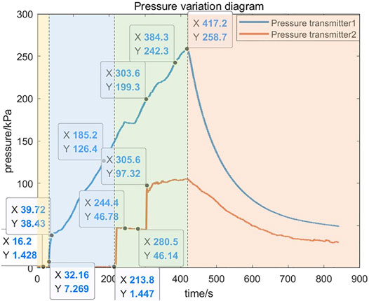
FIGURE 6. Selection of points for power spectrum analysis.

The DC component does not carry useful information with time. The frequency of the DC component is 0, and its power amplitude is generally large. It is inconducive to observe the dynamic changes of other frequency signals with small power amplitude. So, in Table 1, the power spectrum analysis of the acoustic emission signal after removing the DC component is recorded.

TABLE 1

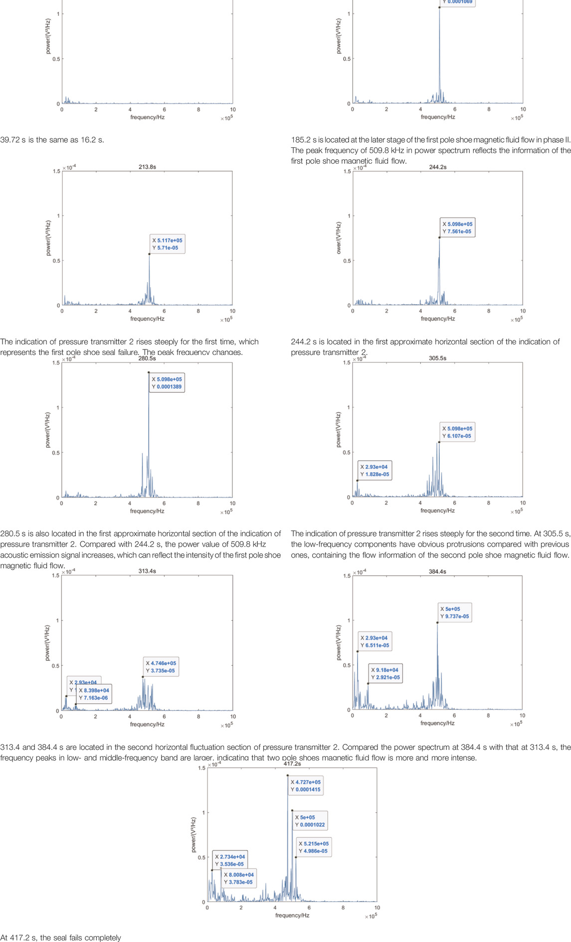
TABLE 1. Power spectrum analysis of the acoustic emission signal.

To sum up, the medium-frequency band contains information about the first pole shoe magnetic fluid flow, and the low-frequency band contains the information about the second pole shoe magnetic fluid flow. The key frequency points include 509.8, 500, and 472.7 kHz in the medium-frequency band and 29.3 kHz in the low-frequency band.

According to the abovementioned key frequency points, bandpass and lowpass Butterworth digital filters are designed to filter acoustic emission signals. The specific parameters are shown in Table 2. The amplitude and phase frequency responses of the filters are shown in Figure 7. The time-domain original and smoothed curves before and after filter processing are shown in Figure 8.

TABLE 2

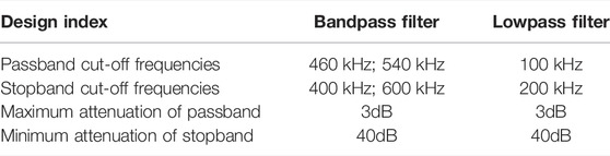
TABLE 2. Designed Butterworth digital filter.

FIGURE 7

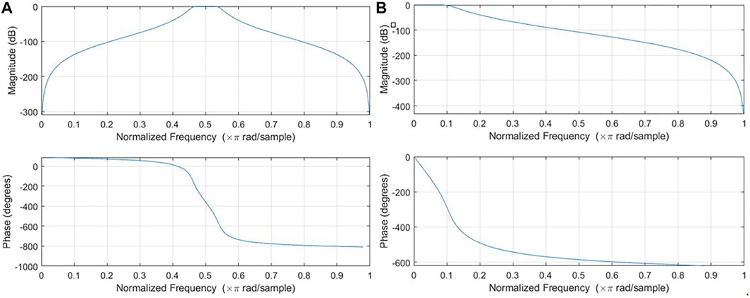
FIGURE 7. Amplitude and phase-frequency response of filters. (A) Bandpass filter.(B) Lowpass filter.

FIGURE 8

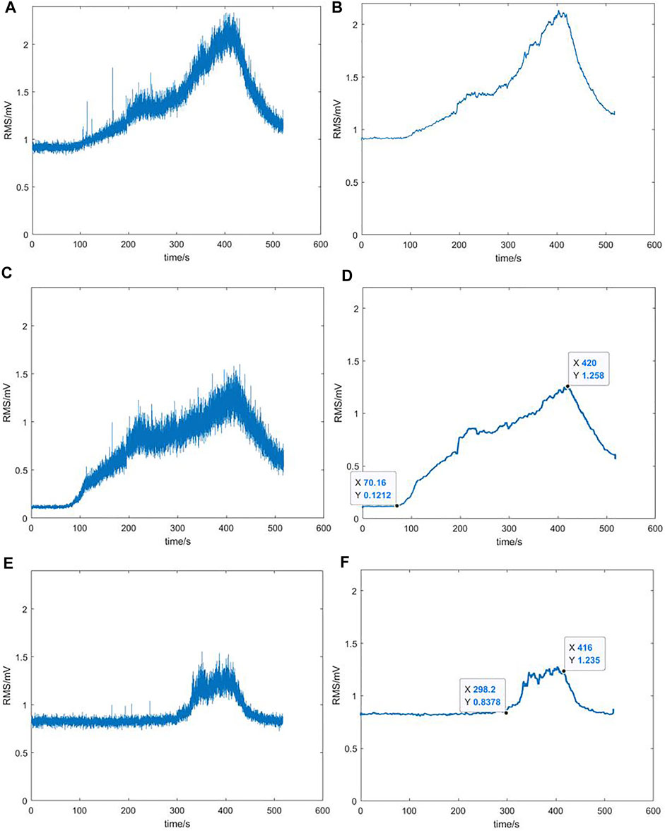
FIGURE 8. Comparison of original and smoothed acoustic emission signal before and after filtering. (A) Original signal. (B) Smoothed signal. (C) Original signal after bandpass filtering. (D) Smoothed signal after bandpass filtering. (E) Original signal after lowpass filtering. (F) Smoothed signal after lowpass filtering.

The signal of the first pole shoe magnetic fluid flow is retained after bandpass filtering (Figure 8D), whose overall trend is consistent with the original (Figure 8B), indicating that it accounts for a large proportion of this experiment. The curve after bandpass filtering shows an upward trend from about 70 s, which means the first pole shoe magnetic fluid begins to flow. The signal’s root mean square (RMS) is not 0 before that because of existing noises. The signal of the second pole shoe magnetic fluid flow and main noises are retained after lowpass filtering (Figure 8F). The curve shows obvious protrusion in 298–416 s, which indicates the second pole shoe magnetic fluid flow at this time. At other times, the curve is approximately horizontal, and the RMS is not 0 because of the stable noises. This curve is quite different from the original one. It means that the proportion of the second pole shoe magnetic fluid flow signal is small in this experiment. Furthermore, the initial distribution of magnetic fluid is uneven.

Therefore, the specific time of two pole shoes magnetic fluid flow can be obtained after power spectral analysis and filtering. The filtered acoustic emission signal’s RMS can reflect the intensity of the magnetic fluid flow. The initial distribution of magnetic fluid under two pole shoes can be inferred from the above mentioned two pole shoes. So, the oil-based magnetic fluid flow information reflected by the acoustic emission signal is richer than the pressure signal.

According to the abovementioned analysis, the process before oil-based magnetic fluid seal failure can be divided into three stages: 0–70.16 s is the first stage, and there is no magnetic fluid flow; 70.16–298.2 s is the second stage, the first pole shoe magnetic fluid flow; and 298.2–416 s is the third stage, two pole shoes magnetic fluid flow together. In order to avoid the inaccuracy of acoustic emission signal sample classification by artificially selecting time points, take 8s before and after the abovementioned time points as the transition period. Therefore, the acoustic emission signal samples collected in 0–62.16 s correspond to the first stage, 78.16–290.2 s correspond to the second stage, and 306.2–408s correspond to the third stage. It will take a long time and low efficiency if all of the acoustic emission data are read and processed. So, we read a sample every 0.04 s using MATLAB in order to correspond well with the pressure data. A total of 9,330 samples are obtained. Among them, there are 1,543 samples in the first stage, 5,261 samples in the second stage, and 2,526 samples in the third stage. The training set and testing set are divided according to the ratio of 2:1, so there are 6,220 training set samples and 3,110 testing set samples.

Flow-State Identification of Oil-Based Magnetic Fluid Seal Based on Random Forest

Feature Extraction

An acoustic emission signal sample $\mathit{X}=\left[x_1,x_2,\dots ,x_N\right]$ is a discrete time series with finite length, and $P\left(f_i\right)$ is the signal’s power value at frequency $f_i$. The common time- and frequency-domain eigenvalues are shown in Tables 3, 4. Those eigenvalues obtained from acoustic emission signal samples form a 21-dimensional eigenvector as input of the subsequent identification model.

TABLE 3

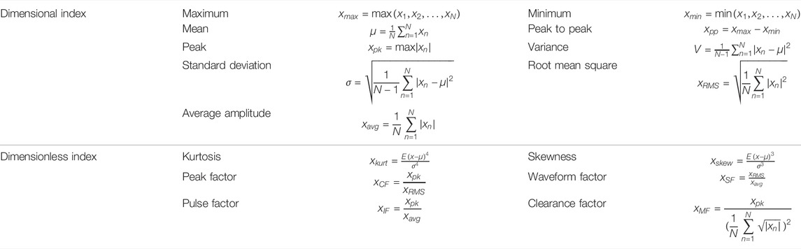
TABLE 3. Calculation formulas of common time-domain eigenvalues.

TABLE 4

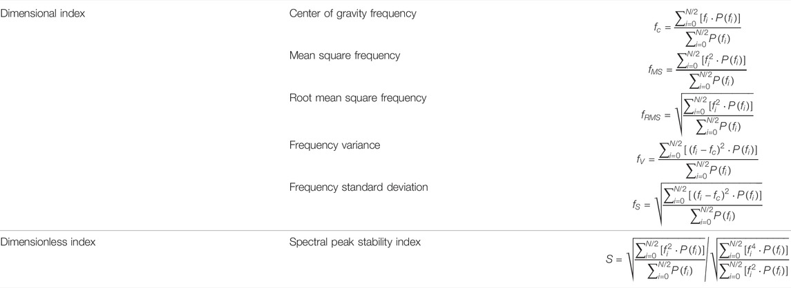
TABLE 4. Calculation formulas of common frequency-domain eigenvalues.

Random Forest Identification Model Based on Grey Wolf Optimizer

Random forest is a supervised learning algorithm that integrates the results of multiple classification and regression trees (CART), as shown in Figure 9. Its specific process is as follows.

1) Construct sub-training samples. Repeat random sampling with putting back (bootstrap sampling) from the original samples to construct sub-training samples.

2) Construct the sub-input eigenvalues set. Randomly sample $mtry$ eigenvalues without putting back from $m(mtry<m)$ originals to construct the sub eigenvalues set as the input of the base classifier.

3) Train CART base classifier. CART is a binary tree as shown in Figure 9. Select the classification eigenvalue at the parent node and classify the samples according to set rules. The leaf node represents the classification result. Since the input eigenvalues in this study are continuous, it is necessary to discretize them by dichotomy. The specific process is shown in Figure 10. $t_i\left(i\in \left[1, l\cdot \left(n-1\right)\right]\right)$ is the selected classification point according to the Gini coefficient, which can reflect the purity of samples in child nodes. The smaller the Gini coefficient, the higher the purity of samples. The Gini coefficient of $t_i$ is defined as

$Gin{i}_{index\left(D_i,t_i\right)}=p_L\left[1-{\displaystyle \sum }_{j=1}^{J}p{\left(k\right)}^2\right]+p_R\left[1-{\displaystyle \sum }_{j=1}^{J}p{\left(k\right)}^2\right],(2)$

where $p_L$ and $p_R$ represent the proportion of samples in the left and right child nodes, respectively. $p\left(k\right)$ represents the proportion of samples belonging to category $j$ in child nodes. The total number of categories is $J$. Select the corresponding eigenvalue $M$ of $t_i$ with the smallest Gini coefficient as the classification eigenvalue of the parent node. The left and right child nodes, respectively, contain samples with $M\le t_i$ and $M>t_i$. In this way, the samples are classified. The training is completed until the sample purity in the child node reaches the maximum or all eigenvalues have been used.

4) Construct a random forest model. Repeat steps (1) (2) (3) and $ntree$ CARTs are generated in parallel to construct a random forest.

5) Output final classification results. In a CART, each path from the root node to a leaf node represents a rule. When testing, the input eigenvalues of the testing sample uniquely determine a path. The category of most samples in this leaf node is the prediction result of the testing sample. The final classification result is determined by the output of $ntree$ CARTs according to the maximum number of votes.

FIGURE 9

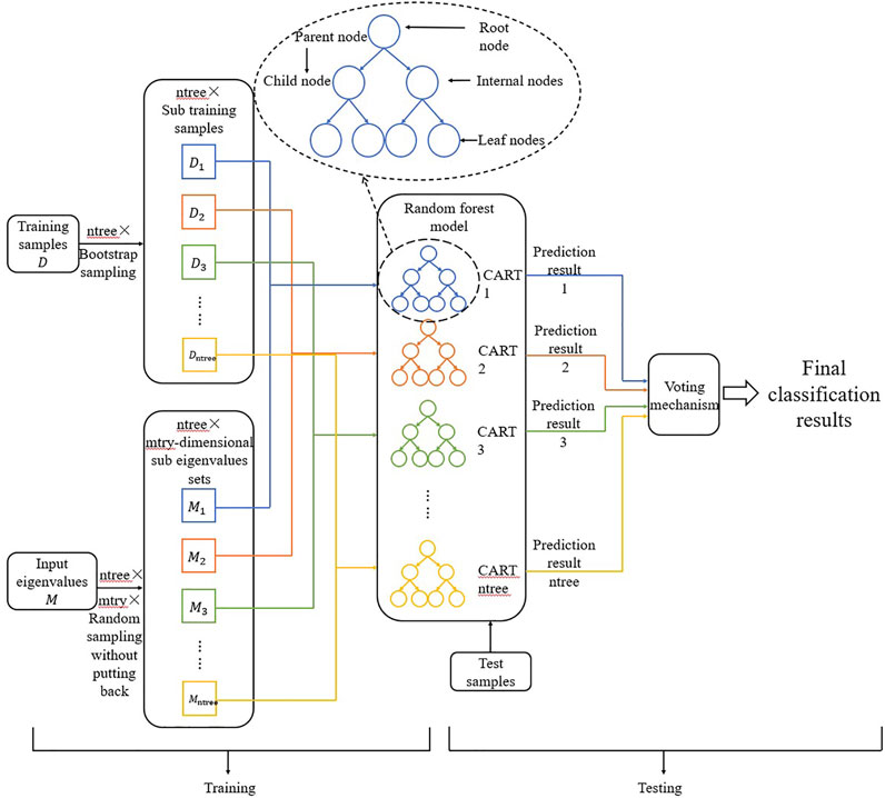
FIGURE 9. Flow diagram of the random forest model.

FIGURE 10

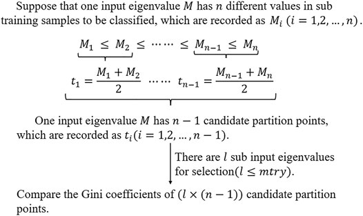
FIGURE 10. Flow diagram of discretized continuous eigenvalues by dichotomy.

$ntree$ and $mtry$ are important to the random forest model’s final classification results (Tan et al., 2022). A grey wolf optimizer (GWO) is used to find the superparameter combination in this study.

GWO is a new swarm intelligence optimization algorithm, which simulates the strict social hierarchy and collective hunting behavior of the grey wolf group. $\alpha ,\beta ,\delta ,\omega$ are four different levels of grey wolves who are distinguished by the fitness values of individuals. The optimal solution is taken as $\alpha$, the second and third are $\beta$ and $\delta$, and the remaining are $\omega$.

The formulas imitating the behavior of wolves surrounding prey are as follows.

$\mathit{D}=\left|\mathit{C}\cdot {\mathit{X}}_p\left(t\right)-\mathit{X}\left(t\right)\right|,(3)$

$\begin{array}{c}\mathit{X}\left(t+1\right)={\mathit{X}}_p\left(t\right)-\mathit{A}\cdot \mathit{D}\end{array},(4)$

where $\mathit{A}$ and $\mathit{C}$ are coefficient vectors; ${\mathit{X}}_p$ and $\mathit{X}$ are the position vector of prey and grey wolf, respectively; $t$ is the current number of iterations; $\mathit{D}$ is the distance between the wolves and prey. $\mathit{A}$ and $\mathit{C}$ are calculated as follows:

$\begin{array}{c}\mathit{A}=2\mathit{a}\cdot {\mathit{r}}_1-\mathit{a}\end{array},(5)$

$\mathit{C}=2\cdot {\mathit{r}}_2,(6)$

where $\mathit{a}$ decreases linearly from 2 to 0 with iteration and ${\mathit{r}}_1$ and ${\mathit{r}}_2$ are random numbers distributed in the interval [0,1] so that grey wolves can move to any position within a certain range around the prey. The encirclement is realized as $\mathit{a}$ decreases to 0. So the value range of $\mathit{A}$ is [-a, a]. When $\left|\mathit{A }\right| < 1$, the wolf will be close to attacking the prey. When $\left|\mathit{A} \right|> 1$, the wolf will be far away to explore. $\mathit{C }$ is the random location weight representing the wolves’ influence on the prey. Its value range is [0,2]. $\mathit{A}$ and C can avoid the algorithm falling into local optimization.

In GWO, $\alpha$, $\beta$, and $\delta$ guide $\omega$ to hunt. The location update formula of wolves is as follows:

$\begin{array}{c}\{\begin{array}{c}{\mathit{D}}_{\alpha }=\left|{\mathit{C}}_1\cdot {\mathit{X}}_{\alpha }-\mathit{X}\left(t\right)\right|\\ {\mathit{D}}_{\beta }=\left|{\mathit{C}}_2\cdot {\mathit{X}}_{\beta }-\mathit{X}\left(t\right)\right|\\ {\mathit{D}}_{\delta }=\left|{\mathit{C}}_3\cdot {\mathit{X}}_{\delta }-\mathit{X}\left(t\right)\right|\end{array}\end{array},(7)$

$\begin{array}{c}\{\begin{array}{c}{\mathit{X}}_1={\mathit{X}}_{\alpha }-{\mathit{A}}_1\cdot {\mathit{D}}_{\alpha }\\ {\mathit{X}}_2={\mathit{X}}_{\beta }-{\mathit{A}}_2\cdot {\mathit{D}}_{\beta }\\ {\mathit{X}}_3={\mathit{X}}_{\delta }-{\mathit{A}}_3\cdot {\mathit{D}}_{\delta }\end{array}\end{array},(8)$

$\begin{array}{c}\mathit{X}\left(t+1\right)=\frac{{\mathit{X}}_1+{\mathit{X}}_2+{\mathit{X}}_3}{3}\end{array},(9)$

where ${\mathit{D}}_{\alpha }$, ${\mathit{D}}_{\beta }\mathrm{,}{\mathit{D}}_{\delta }$, respectively, represent the distances from $\alpha \mathrm{,}\beta \mathrm{,}\delta$ to other individuals; ${\mathit{X}}_{\alpha }\mathrm{,}{\mathit{X}}_{\beta }\mathrm{,}{\mathit{X}}_{\delta }$, respectively, represent the current location of $\alpha \mathrm{,}\beta \mathrm{,}\delta$; $X\left(t\right)$ is the current location of the grey wolf. Formula (8) defines step and direction for $\omega$ move on to $\alpha \mathrm{,}\beta \mathrm{,}\delta$. Formula (9) defines $\omega$’s final position.

In this study, the acoustic emission signal sample’s time- and frequency-domain eigenvalues are extracted as the input to train GWO_RF model identifying the oil-based magnetic fluid flow state before seal failure.

Identification Result

Train the random forest model by the function classRF_train () in MATLAB R2018b. Apply GWO to optimize two super parameters of $ntree$ and $mtry$. The number of grey wolf population and iterations are both 10. Optimize $ntree$ in [1,100] and $mtry$ in [1,21]. Take the classification accuracy of the testing set as the fitness. The confusion matrixes of 10 times training results are shown in Figure 11.

FIGURE 11

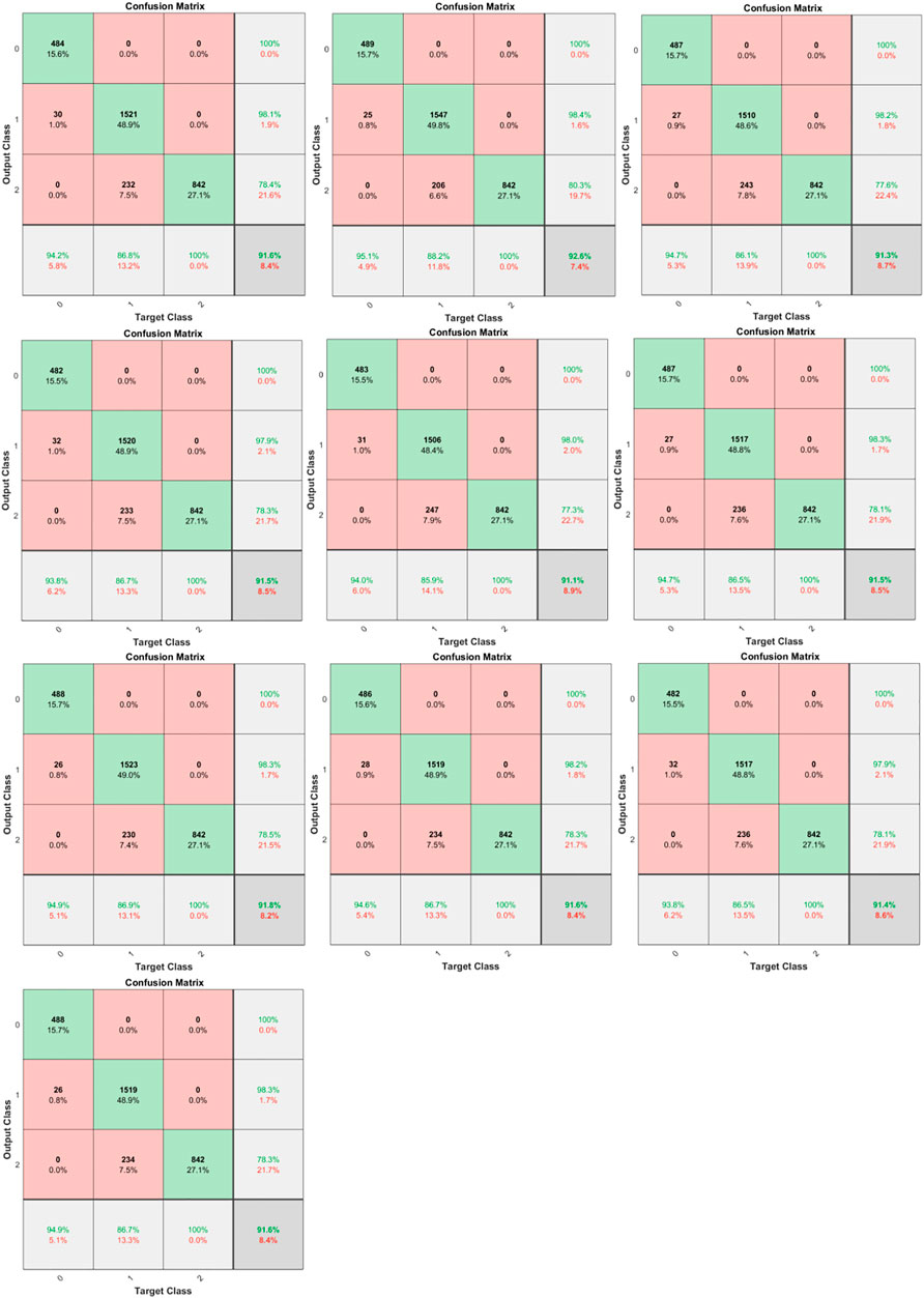
FIGURE 11. Confusion matrixes of 10 times’ training results.

In the confusion matrix, the row corresponds to the prediction class, the column corresponds to the real class, the diagonal unit corresponds to correct classification, and the non-diagonal unit corresponds to wrong classification. The number and the percentage are displayed in each cell. The rightmost column of the chart shows the correct and wrong classification in the prediction results, which are called precision and error detection rates, respectively. The row at the bottom of the chart shows the ones in the real category, which are called recall rate and false-negative rate. The cell at the bottom right of the chart shows overall accuracy. The confusion between “the first pole shoe magnetic fluid flow” and “two-pole shoes magnetic fluid flow” is serious.

Only the accuracy value is not suitable for evaluating the models with large quantity deviation in different categories of samples. In theory, the higher the precision and recall rate, the better. But they are often inconsistent. The F score is often used to consider them comprehensively. Its calculation formula is as follows:

$F=\frac{\left(a^2+1\right)\ast P\ast R}{a^2\ast \left(P+R\right)},(10)$

where P: precision, R: recall, $a$: weight factor. When $a = 1$, it changes to the most common evaluation index F1 score, representing the weight of precision and recall are the same. Its calculation formula is

$F1=\frac{2\ast P\ast R}{P+R}.(11)$

Table 5 summarizes the GWO_RF model’s 10 training results. The last line is the average of them. It can be found that F1 scores of three oil-based magnetic fluid flow states before seal failure are close to or greater than 90%, among which, the F1 score of “two pole shoe magnetic fluid flow” is relatively low. The F1 scores obtained from each training are similar although the optimization results have great randomness. Of course, GWO takes a long time to optimize the parameters.

TABLE 5

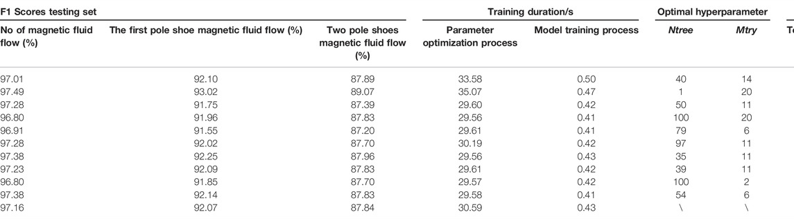
TABLE 5. Information statistics of GWO_ RF model.

Conclusion

In this study, nondestructive acoustic emission testing technology is proposed to monitor the oil-based magnetic fluid flow state before the seal failure so as to speculate the seal performance. The experiment is designed to collect the acoustic emission and pressure signals at the same time. The acoustic emission signal is analyzed and filtered assisted by the pressure signal. The process before the oil-based magnetic fluid seal failure is divided into three stages: no magnetic fluid flow, the first pole shoe magnetic fluid flow, and two pole shoe magnetic fluid flow together, and the acoustic emission signal samples are classified. Extract the time- and frequency-domain eigenvalues forming a 21-dimensional eigenvector as the input and train the random forest model based on grey wolf optimizer to optimize the $ntree$ and $mtry$. The testing accuracy and F1 scores of the three states are close to or higher than 90%, indicating the feasibility of acoustic emission technology and the effectiveness of spectrum analysis and filtering for the acoustic emission signal to distinguish three flow states. In future studies, we can redesign the structure of the seal element, which can measure the pressure change between each two pole teeth. So we can analyze the acoustic emission signal more accurately with the help of more detailed pressure signals. Also, we can compare acoustic emission signals with the changing of parameters such as shaft rotation speed and temperature under dynamic conditions.

Data Availability Statement

The original contributions presented in the study are included in the article/Supplementary Material; further inquiries can be directed to the corresponding author.

Ethics Statement

Ethical review and approval was not required for the study on human participants in accordance with the local legislation and institutional requirements. The patients/participants provided their written informed consent to participate in this study.

Author Contributions

Conceptualization: JX, YX, and DL; methodology: JX and YX; software: JX; validation: JX and YX; resources: DL; data curation: JX; writing—original draft preparation, JX; writing—review and editing: YX and DL; supervision: DL; project administration: DL. All authors have read and agreed to the published version of the manuscript.

Funding

This work was supported by the National Natural Science Foundation of China (grant numbers: 51735006, U1837206, 51927810) and the Beijing Municipal Natural Science Foundation (grant number: 3182013).

Conflict of Interest

The authors declare that the research was conducted in the absence of any commercial or financial relationships that could be construed as a potential conflict of interest.

Publisher’s Note

All claims expressed in this article are solely those of the authors and do not necessarily represent those of their affiliated organizations, or those of the publisher, the editors, and the reviewers. Any product that may be evaluated in this article, or claim that may be made by its manufacturer, is not guaranteed or endorsed by the publisher.

Acknowledgments

We acknowledge the resources provided by the laboratory and the guidance of all teachers.

Supplementary Material

The Supplementary Material for this article can be found online at: https://www.frontiersin.org/articles/10.3389/fmats.2022.930885/full#supplementary-material

References

Chen, Y. B. (2019). Study on Magnetic Fluid Seals under High Speed Condition. Doctoral Dissertation. Beijing: University of Science and Technology Beijing. Available at: https://kns.cnki.net/KCMS/detail/detail.aspx?dbname=CDFDLAST2019&filename=1019157279.nh.

Google Scholar

Ge, Z. D., Fu, P., and Zhang, E. Q. (2016). Monitoring Technique of Film Seal Face Friction Condition Based on Kalman Filtering. Lubr. Eng. 41 (04), 106–110. Available at: https://kns.cnki.net/kcms/detail/detail.aspx?FileName=RHMF201604027&DbName=CJFQ2016.

Google Scholar

Jiang, Y. (2015). The Monitoring Research on the Open Process of Hydrodynamic Mechanical Seals Based on Acoustic Emission Characteristics. Master Degree Dissertation. Chengdu, Sichuan: Southwest Jiaotong University. Available at: https://kns.cnki.net/KCMS/detail/detail.aspx?dbname=CMFD201601&filename=1015338185.nh.

Google Scholar

Kurfess, J., and Müller, H. K. (1990). Sealing Liquids with Magnetic Liquids. North-Holland 85 (1-3). doi:10.1016/0304-8853(90)90059-y

CrossRef Full Text | Google Scholar

Li, D. C., and Hao, D. (2018). Major Problems and Solutions in Applications of Magnetic Fluid Rotation Seal. Chin. J. Vac. Sci. Technol. 38 (07), 564–574. doi:10.13922/j.cnki.cjovst.2018.07.04

CrossRef Full Text | Google Scholar

Li, X. H., Fu, P., and Zhang, Z. (2014). Measurement of Film Thickness in Mechanical Seals Based on AE Technology. Adv. Eng. Sci. 46 (06), 198–204. doi:10.15961/j.jsuese.2014.06.031

CrossRef Full Text | Google Scholar

Li, X. H. (2016). Hydrodynamic Mechanical Seal End Faces Condition Monitoring and Health Assessment. Doctor Degree Dissertation. Chengdu, Sichuan: Southwest Jiaotong University. Available at: https://kns.cnki.net/KCMS/detail/detail.aspx?dbname=CDFDLAST2018&filename=1017298548.nh.

Google Scholar

Li, Y. F. (2017). “Study on Condition Monitoring and Performance Evaluating System of Liquid Film Seals,” in Degree Thesis of Engineering Master. China University of Petroleum (East China). Available at: https://kns.cnki.net/KCMS/detail/detail.aspx?dbname=CMFD201902&filename=1019838884.nh.

Google Scholar

Sun, X. H., Dong, X. W., Zhang, T. F., Hao, M. M., Cao, H. C., Wang, Y. L., et al. (2018). Research Progress of Acoustic Emission in Seal Monitoring. Lubr. Eng. 43 (06), 136–140. Available at: https://kns.cnki.net/kcms/detail/detail.aspx?FileName=RHMF201806025&DbName=CJFQ2018. 10.2478/pomr-2018-0122.

Google Scholar

Tan, C. Y., Zhang, Z. S., Zhou, X. Q., Guo, J. H., Xiao, H., Chen, T., et al. (2022). Pattern Recognition Model of Coalbed Methane Productivity Based on Random Forest Algorithm. Saf. Coal Mines 53 (02), 170–178+186. doi:10.13347/j.cnki.mkaq.2022.02.027

CrossRef Full Text | Google Scholar

Wang, Z. Z. (2019). The Study of Sealing Liquid with Magnetic Fluid. Doctoral Dissertation. Beijing: Beijing Jiaotong University. Available at: https://kns.cnki.net/KCMS/detail/detail.aspx?dbname=CDFDLAST2020&filename=1019210031.nh.

Google Scholar

Zhang, E. Q. (2015). Research of Key Technologies on Mechanical Seal End Face Condition Monitoring and Life Prediction. Doctor Degree Dissertation. Chengdu, Sichuan: Southwest Jiaotong University. Available at: https://kns.cnki.net/kcms/detail/detail.aspx?FileName=1016177215.nh&DbName=CDFD2016

Google Scholar

Zhang, F. (2016). Research on Fault Diagnosis Method for Rotating Machine Based on LMD and HSMM. Master Degree Thesis. Chengdu, Sichuan: Southwest Jiaotong University. Available at: https://kns.cnki.net/kcms/detail/detail.aspx?FileName=1016155076.nh&DbName=CMFD2016.

Google Scholar