 Jiwei Zhang
 Jing Lu
 Feng Chen3
- 1School of Mathematics and Statistics, Yunnan University, Kunming, China
- 2School of Mathematics and Statistics, Northeast Normal University, Changchun, China
- 3Department of East Asian Studies, The University of Arizona, Tucson, AZ, United States
In many large-scale tests, it is very common that students are nested within classes or schools and that the test designers try to measure their multidimensional latent traits (e.g., logical reasoning ability and computational ability in the mathematics test). It is particularly important to explore the influences of covariates on multiple abilities for development and improvement of educational quality monitoring mechanism. In this study, motivated by a real dataset of a large-scale English achievement test, we will address how to construct an appropriate multilevel structural models to fit the data in many of multilevel models, and what are the effects of gender and socioeconomic-status differences on English multidimensional abilities at the individual level, and how does the teachers' satisfaction and school climate affect students' English abilities at the school level. A full Gibbs sampling algorithm within the Markov chain Monte Carlo (MCMC) framework is used for model estimation. Moreover, a unique form of the deviance information criterion (DIC) is used as a model comparison index. In order to verify the accuracy of the algorithm estimation, two simulations are considered in this paper. Simulation studies show that the Gibbs sampling algorithm works well in estimating all model parameters across a broad spectrum of scenarios, which can be used to guide the real data analysis. A brief discussion and suggestions for further research are shown in the concluding remarks.
1. Introduction
With the increasing interest in multidimensional latent traits and the advancement in estimation techniques, multidimensional item response theory (IRT) has been developed vigorously which made the model estimation become easy to implement and effective. Single-level multidimensional IRT (MIRT) models were proposed decades ago, as it have the primary features of modeling the correlations among multiple latent traits and categorical response variables (Mulaik, 1972; Reckase, 1972, 2009; Sympson, 1978; Whitely, 1980a,b; Way et al., 1988; Ackerman, 1989; Muraki and Carlson, 1993; Kelderman and Rijkes, 1994; Embretson and Reise, 2000; Béguin and Glas, 2001; Yao and Schwarz, 2006). The MIRT models later incorporated covariates to elucidate the connection between multiple latent traits and predictors (Adams et al., 1997; van der Linden, 2008; De Jong and Steenkamp, 2010; Klein Entink, 2009; Klein Entink et al., 2009; Höhler et al., 2010; Lu, 2012; Muthén and Asparouhov, 2013).
It has become frequent practice to regard IRT model calibration's latent ability as a dependent variable in resulting regression analysis in relation to educational and psychological measurement. Measurement error within latent ability estimates is ignored in this two-stage treatment resulting in statistical inferences that may be biased. Specially, measurement error can reduce the statistical power of impact studies and deteriorate the researchers' ability to ascertain relationships among different variables affecting student outcomes (Lu et al., 2005). One error that can reduce the statistical capabilities of impact studies and make it difficult for researchers to identify relationships between variables related to student outcomes is the measurement error.
Taking a multilevel perspective on item response modeling can avoid issues that arise when analysts use latent regression (using latent variables as outcomes in regression analysis) (Adams et al., 1997). The student population distribution is commonly handled as a between-student model with the IRT model being placed at the lowest level as a within-subject model within the structure of multilevel or hierarchical models. Using a multilevel IRT model gives analysts the ability to estimate item and ability parameters along with structural multilevel model parameters at the same time (e.g., Adams et al., 1997; Kamata, 2001; Hox, 2002; Goldstein, 2003; Pastor, 2003). This results in measurement error associated with estimated abilities being accounted for when estimating the multilevel parameters (Adams et al., 1997).
Although the multilevel IRT models have been deeply studied in the last 20 years, there are significant differences between our multilevel IRT models and the existing literatures in the problem to be solved and the viewpoint of modeling. Next, we discuss the differences from many aspects. Multidimensional IRT models that have a hierarchical structure relationship between specific ability and general ability were developed in 2007 by Sheng and Wikle. Specifically, general ability has a linear relationship with specific ability, or all specific abilities linearly combine within a general ability. However, the hierarchical structure in our study refers to the nested data structure, for example, the students are nested in classes while classes are nested in schools, rather than the hierarchical relationships between specific ability and general ability. The modeling method similar to Sheng and Wikle (2007) also includes Huang and Wang (2014) and Huang et al. (2013). Note that in Huang and Wang (2014), not only the hierarchical abilities models are discussed, but also the multilevel data are modeled. Muthén and Asparouhov (2013) proposed the multilevel multidimensional IRT models to investigate elementary student aggressive-disruptive behavior in school classrooms and the model parameters were estimated in Mplus (Muthén and Muthén, 1998) using Bayes. Although Muthén and Asparouhov (2013) and our current study also focus on the multilevel multidimensional IRT modeling, there are great differences in the model construction. In the multilevel modeling, they suggested that the ability (factor) of each dimension has between-and within-cluster variations. However, the sources of the between—and within—cluster variations are not taken into account. More specifically, whether these two types of variation are affected by the between cluster covariates and within individual background variables have not been further analyzed. Similarly, in the works of both Höhler et al. (2010) and Lu (2012) demonstrated the same modeling method. In our study, the between—and within—cluster variations are further explained by considering the effects of individual and school covariates on multiple dimensional latent abilities. For example, we can consider whether the gender difference between male and female has an important influence on the vocabulary cognitive ability and reading comprehension ability. Moreover, Chalmers (2015) proposed an extended mixed-effects IRT models to analyze PISA data. By using a Metropolis-Hastings Robbins-Monro (MH-RM) stochastic imputation algorithm (cf. Cai, 2010a,b,c, 2013), it evaluates fixed and random coefficients. Rather than directly explaining the multiple dimensional abilities, the individual background (level-1) and school (level-2) covariates are used to model the fixed effects.
In order to illustrate the interactions between unidimensional ability and individual—and school—level covariates where the ability parameters possess a hierarchical nesting structure, Fox and Glas (2001) and Kamata (2001) proposed multilevel IRT models. In this current research, we broaden Fox and Glas (2001) and Kamata (2001)'s models by swapping their unidimensional IRT model with a multidimensional normal ogive model because we want to assess students' four types of abilities from a large-scale English achievement test. We particularly pay attention to investigating the connection between multiple latent traits and covariates. Taking the proposed multilevel multidimensional IRT models as the basis, the following issues will be addressed. (1) According to the model selection results, which model is the best to fit the data and how can judge the individual-level regression coefficients be judged as fixed effect or random effect? (2) How will students from different ends of the socioeconomic-status (SES) score in English performance as tested in four types of latent abilities, based on the level-2 gender (GD), level-3 teacher satisfaction (ST) and school climate (CT) [The details of the Likert questionnaires for measuring teacher satisfaction and school climate, please refer to (Shalabi, 2002)]. (3) What relationship exists between males and females' performances in different latent abilities by controlling for SES, ST and CT. (4) What effects, if any, are seen with different teachers' or schools' effects (covariates)? (5) Is it possible to use a measurement tool to determine whether items' factor patterns correlate to the subscales of the test battery? In particular, will the four subtests of the test battery be discernable according to the discrimination parameters on the four dimensions?
The rest of the article is organized as follows. Section 2 presents the detailed development of the proposed multilevel multidimensional IRT models and procedure for hierarchical data. Section 3 provides a Bayesian estimation method to meet computational challenges for the proposed models. Meanwhile, Bayesian model assessment criteria is discussed in section 3. In section 4, simulation studies are conducted to examine the performances of parameter recovery using the Gibbs sampling algorithm. In addition, a real data analysis of the education quality assessment is given in section 5. We conclude this article with a brief discussions and suggestions for further research in section 6.
2. Multilevel Multidimensional IRT Model
The model contains three levels. At the first level, a multidimensional normal ogive IRT model is defined to model the relationship between items, persons, and responses. At the second level, personal parameters are predicted by personal-level covariates, such as an individual's social economic status (SES). At the third level, persons are nested within schools, and school-level covariates are included such as school climate and teacher satisfaction.
• The measurement model at level 1 (multidimensional two parameter normal ogive model; Samejima, 1974; McDonald, 1999; Bock and Schilling, 2003)
In terms of notation, let j = 1, …, J indicate J schools (or groups), and within school j, there are i = 1, …, nj individuals. The total number of individuals is n = n1 + n2 +… + nJ. k = 1, …, K indicate the items. In Equation (2.1), Yijk denotes the response of the ith individual in the jth group answering the kth item. The corresponding correct response probability can be expressed as pijk, and θij denotes a Q-dimensional vectors of ability parameters for the ith individual in the jth group, i.e., and denotes the vector of item parameters, in which ak = is a vector of discrimination or slope parameters, and bk is the difficulty or intercept parameter. Let The latent abilities of different dimensions can be explained by individual-level background covariates. Note that the multidimensional IRT model used in this paper actually belongs to the within-items multidimensional IRT model. That is, each item measures multiple dimensional abilities, and each test item has loadings on all these abilities. Unlike the between-items multidimensional IRT model, each item has a unity loading on one dimensional ability and zero loadings on other dimensional abilities. For a further explanation of the model used in this paper, please see Table 1 in the following simulation study 1.
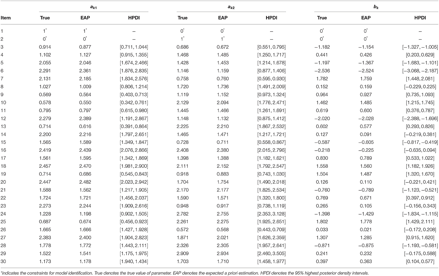
Table 1. Estimation of simulated item parameter estimation using Gibbs sampling algorithm in simulation study 1.
• Multilevel structural model at level 2 (individual level) can be represented by
In Equation (2.2), the level-2 individual covariates are denoted as Xij = (x1ij, x2ij, …, xhij), where h is the number of individual background covariates. Xij can contain both continuous and discrete variables (e.g., socio-economic status, gender). The residual term, is assumed to follow a multivariate normal distribution N(0, Σe). Here, Σe is a Q-by-Q variance-covariance matrix. The individuals' abilities are considered to be the latent outcome variables of the multilevel regression model. Differences in abilities among individuals within the same school are modeled given student-level characteristics. Therefore, the explanatory information Xij at the individual level explains variability in the latent abilities within school.
• Level 3 (school level) model in this current study can be expressed as follows:
In Equation (2.3), the level-3 school covariates are represented by , where s is the number of school covariates at level 3. Each level-2 random regression coefficient parameter is βhjq, which can be interpreted by school level covariates. The level-3 residual is multivariate normally distributed with mean 0 and (h + 1)-by-(h + 1) covariance matrix Tq, q = 1, …, Q. The variation across schools is modeled given background information at the school level. To control the model complexity, we assume that the level-3 residual covariance between different dimensions is 0; that is
Different from Equation (2.2) in this paper, Huang and Wang (2014) proposed a high-order structure model to construct ability parameters with hierarchical strucutre. More specifically, all specific abilities linearly combine within a general ability. Assuming that there are two order of ability, including and , their relationship is described by the following model
where and denote first-order ability and second-order ability for the ith student sampled from school v, the subscript q denotes the dimension of the first-order ability. β0qv, β1qv, and are the intercept, slope, and residual for the qth first-order ability in the vth school, respectively. is the within-school residual and is typically assumed to be homogeneous across schools and normally distributed with a mean of zero and a variance of and independent of the other ε and θ. However, in this current study, we only focus on the specific abilities of four dimensions without the general ability, which is the different between Huang and Wang (2014) and us in the construction of the ability structure model.
Moreover, in Huang and Wang (2014)'s paper, the multilevel data structure is investigated by introducing the individual level predictions directly into the above-mentioned higher-order ability model (Equation 2.5). The specific model is as follows:
where Ghiv is the hth individual level predictor for the ith student in the vth school and βhqv is its corresponding regression weight for the qth ability and school v. At the school level, the random coefficients β can be modeled as
where h = 2, …, H, and the residuals are assumed to follow a multivariate normal distribution with a mean vector of zero and a covariance matrix of Σu. Further, school level predictors (e.g., school type, school size) can be added to the random intercept model. That is,
where Wkv is the kth school level predictor and γkv is its corresponding regression weight for the qth ability.
However, in this current study, the multiple dimensional abilities are directly built into the random regression models through the individual level predictors (Equation 2.2). It is not the same as Huang and Wang (2014, p. 498, Equation 4) that constructs hierarchical structure ability and multilevel data in one model. In addition, when constructing the school level models in our paper, school level predictive variables, such as teacher satisfaction, school climate, are used to model the random intercept and random slopes (Equation 2.3). Considering if different predictors are added to the school level model, multiple versions of the school level models are generated. Therefore, we can use the Bayesian model assessment to select the best-fitting model. However, Huang and Wang (2014) only model the random intercept by predictive variables at school level, without considering the impact of predictive variables on other random coefficients (page 498, Equation 8).
3. Bayesian Parameter Estimation and Model Selection
3.1. Identifying Restrictions
In this current study, the multilevel multidimensional IRT models are identified based on discrimination and difficulty parameters (Fraser, 1988; Béguin and Glas, 2001; Skrondal and Rabe-Hesketh, 2004). The most convenient method is to set Q item parameters bk equal to 0 if k = q, and impose the restrictions akq = 1, where k = 1, 2, …Q, and q = 1, …, Q. If k ≠ q, akq = 0. If k > q, bk and akq will be free parameters to estimate. The basic idea is to identify the model by anchoring several item discrimination parameters to an arbitrary constant, typically akq = 1. Meanwhile, the location identification constrains is required by restricting the difficulty parameters for given items, typically, bk = 0. Based on the fixed anchoring values of item parameters, other parameters are estimated on the same scale. The estimated difficulty or discrimination values of item parameters are interpreted based on their relative positions to the corresponding anchoring values (Béguin and Glas, 2001, p. 545). Additionally, in order to have a clear understanding of the process of restricting the identifiability, we illustrate the identifiability of the two-dimensional models. For details, please refer to item 1 and item 2 in Tables 1, 2 for the restrictions of discrimination and difficult parameters.
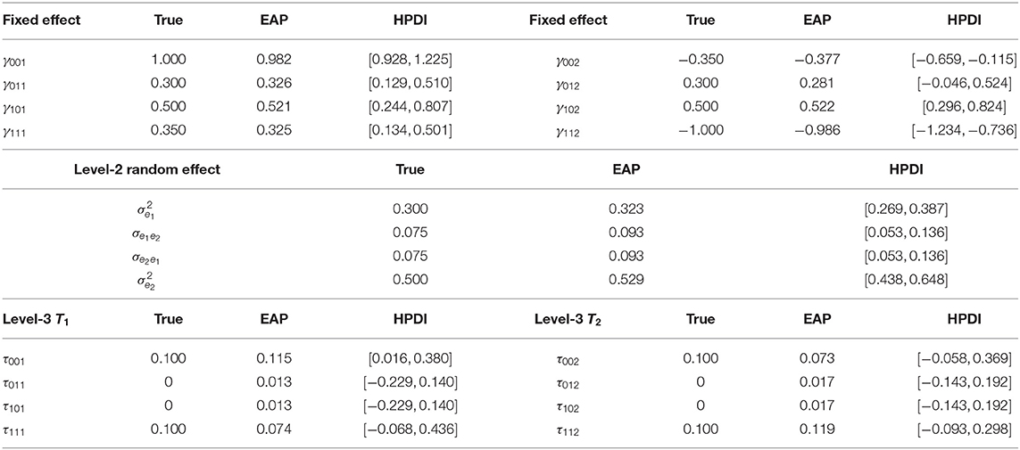
Table 2. Parameter estimates of the fixed effect, Level-2 variance-covariance and Level-3 variance-covariance in simulation 1.
3.2. Gibbs Sampling Within the MCMC Framework
In the framework of frequentist, two commonly used estimation methods are used to estimate the complex IRT models. One is the marginal maximum likelihood estimation (MMLE; Bock and Aitkin, 1981), and the other is the weighted least squares means and variance adjusted (WLSMV; Muthén et al., 1997). However, the main disadvantage of the marginal maximum likelihood method is that it inevitably needs to approximate the tedious multidimensional integral by using numerical or Monte Carlo integration, which will increase large the computational burden. Another disadvantage of the MMLE are that it is difficulty to incorporate uncertainty (standard errors) into parameter estimates (Patz and Junker, 1999a), and the comparison method of the MMLE is simplistic, except the RMSEA (Root Mean Square Error of Approximation) which is often used, other comparison methods are seldom used. In addition, there are some disadvantages in WLSMV compared with Bayesian method used in this paper. Firstly, Bayesian method outperforms WLSMV solely in case of strongly informative accurate priors for categorical data. Even if the weakly informative inaccurate priors are used when the sample size is moderate and not too small, the performance of Bayesian method does not deteriorate (Holtmann et al., 2016). Secondly, compared with WLSMV, Bayesian method does not rely on asymptotic arguments and can give more reliable results for small samples (Song and Lee, 2012). Thirdly, Bayesian method allows the possibility to analyze models that are computationally heavy or impossible to estimate with WLSMV (Asparouhov and Muthén, 2012). For example, the computational burden of the WLSMV becomes intensive especially when a large number of items is considered. Fourth, Bayesian method has a better convergence rate compared with WLSMV. Fifth, Bayesian method can be used to evaluate the plausibility of the model or its general assumptions by using posterior predictive checks (PPC; Gelman et al., 1996). For the above-mentioned reasons, Bayesian method is chosen for estimating the following multilevel multidimensional IRT models.
In fact, Bayesian methods have been widely applied to estimate parameters in complex multilevel IRT models (e.g., Albert, 1992; Bradlow et al., 1999; Patz and Junker, 1999a,b; Béguin and Glas, 2001; Rupp et al., 2004). Within the framework of Bayesian, a series of BUGS softwares can be used to estimate these multilevel IRT models, including OpenBUGS (Spiegelhalter et al., 2003) and JAGS (Plummer, 2003). However, in this paper, we implement the Gibbs sampling by introducing the augmented variables rather than by constructing an envelope of the log of the target density as in a series of BUGS softwares. The auxiliary or latent variable approach has several important advantages. First, the approach is very flexible and can handle almost all sorts of discrete responses. Typically, the likelihood of the observed response data has a complex structure but the likelihood of the augmented (latent) data has a known distribution with convenient mathematical properties. Second, conjugate priors, where the posterior has the same algebraic form as the prior, can be more easily defined for the likelihood of the latent response data, which has a known distributional form, than for the likelihood of the observed data. Third, the augmented variable approach facilitates easy formulation of a Gibbs sampling algorithm based on data augmentation. It will turn out that by augmenting with a latent continuous variable, conditional distributions can be defined based on augmented data, from which samples are easily drawn. Fourth, the conditional posterior given augmented data has a known distributional form such that conditional probability statements can be directly evaluated for making posterior inferences. The likelihood of the augmented response data is much more easily evaluated than the likelihood of the observed data and can be used to compare models. In summary, in this study, we adopt the Gibbs sampling algorithm (Geman and Geman, 1984) with data augmentation (Tanner and Wong, 1987) to estimate multilevel multidimensional IRT models. In particular, let θ and ξ denote the vectors of all person and item parameters. Define an augmented variable Zijk that is normally distributed with mean and variance 1.
The joint posterior distribution of the parameters given the data is as follows:
where is the conditional variance given the other ability dimensions. It can be obtained from Σe. The details of the Gibbs sampling are shown as follows
Step 1: Sampling Z given the parameters θ and ξ, where the random variable Zijk is independent
Step 2: Sampling θij according to Gibbs sampling characteristics. A divide-and-conqueror strategy is used to draw each sampling element of where θij(−1) = (θij2, ···, θijQ). Let where and The conditional prior distribution of θij1 can be written as
Therefore, the full conditional posterior density of θij1 (Lindley and Smith, 1972; Box and Tiao, 1973) is given by
where
For q = 2, …, Q, θijq can be drawn in the same manner.
Step 3: Sampling ξk, Given Here n (n = n1 + n2 + ··· + nJ) represents the total number of individuals in different groups. The residual can be written as εk and each element is distributed as N(0, 1). Therefore, we have
Let H = [θ − 1], the likelihood function of ξk is normally distributed with mean and . Suppose that the priors of the discrimination and difficult parameters are ak ~ N(μa, Σa) I (ak|akq > 0, q = 1, …, Q) and , respective, Here and . The prior of item parameter ξk is a multivariate normal distribution with mean and . Therefore, the full conditional posterior distribution of the item parameters is given by
Step 4: Sampling βj= given θ, γ and T. Dawn an element of vector βj, Let and with Xij as defined in the part of model introduction. The level-2 residual ej1 can be defined as Therefore, we have
The level-2 likelihood function of βj1 is normally distributed with mean and variance . Furthermore, wj is the direct product of wjs = (1, wj1, …, wjs) and a (h + 1) identity matrix, that is, wj = I(h + 1) ⊗ wjs. The random regression coefficient βj1 is induced by a normal prior at level 3 with mean wjγ1 and covariance T1, where The level-3 residual uj1 can be defined as Therefore, we have
Thus, the fully conditional posterior distribution of βj1 is given by
and βjq, q = 2, …, Q, is drawn in the same manner.
Step 5: Sampling γ, γ = (γ1, ···, γQ). An element of vector γ is drawn, and the matrix γ1 is the matrix of regression coefficients corresponding to the regression of βj1 on wj. An improper noninformative prior density for γ1 is used. Similar prior is used as shown in Fox and Glas (2001). Therefore, the full conditional posterior distribution of γ1 is given by
and γq is drawn in the same manner for q = 2, ···, Q.
Step 6: Sampling the residual variance-covariance structure Σe. A prior for Σe is an Inverse-Wishart distribution. The full conditional posterior distribution of Σe is given by
where where N = J × nj.
Step 7: Sampling the level-3 variance-covariance structure T = diag (T1, ···, TQ). T1 is drawn first. A prior for T1 is an Inverse-Wishart distribution. The full conditional posterior distribution of T1 is given by
where and Tq is drawn in the same manner for q = 2, ···, Q.
3.3. Model Selection
The deviance information criterion (DIC) was introduced by Spiegelhalter et al. (2002) as a model selection criterion for the Bayesian hierarchical models. Similar to many other criteria (such as the Bayesian information criterion or BIC; BIC is not intended to predict out-of-sample model performance but rather is designed for other purposes, we do not consider it further here (Gelman et al., 2014), it trades a measure of model adequacy against a measure of complexity. Specifically, the DIC is defined as the sum of a deviance measure and a penalty term for the effective number of parameters based on a measure of model complexity. The model with a larger DIC has a better fit to the data. In the framework of a multilevel IRT models, the performances of DICs based on five versions of deviances have been investigated in Zhang et al. (2019). The DIC used in this current study belongs to the top-level marginalized DIC in their paper. The reason for using the top-level marginalized DIC in our paper is that our main purpose is to investigate the influences of fixed effects (γ) on the multiple dimensional abilities. Therefore, the deviance is defined at the highest level fixed effects (γ), where the random effects of intermediate processes, such as the second-level random individual ability effects θ or the third-level random coefficient effects β, will not be considered in the defined deviance. Next, the calculation formula of the top-level marginalized DIC is given.
Let Ω1 = (ξ, Σe, T) (Ω1 do not include the intermediate process random parameters θ and β). According to the augmented data likelihood p(Z|Ω1), we can obtain the following deviance
Then the top-level marginalized DIC is defined as
In Equation (3.9), the conditional DIC is a function of Z and Ω1, which can be written as [DIC|Z, Ω1]. denotes the deviance of the posterior estimation mean given augmented data Z and Ω1. pD(Z, Ω1) is the effective number of parameters given the augmented data Z and Ω1, which can be expressed as .
An important advantage of DIC is that it can be easily calculated from the generated samples. It can be obtained by MCMC sampling augmentation auxiliary variable Z and structural parameters Ω1 from the joint posterior distribution p(Z, Ω1|Y).
4. Simulation
4.1. Simulation 1
A simulation study is conducted to evaluate the performance of the proposed Gibbs sampler MCMC method for recovering the parameters of the multilevel IRT models. For illustration purposes, we only consider one explanatory variable on both levels, and the number of dimensions is fixed at 2 (q = 2). The true structural multilevel model is simplified as
The individual-level model:
where
The school-level model:
where
We use the multidimensional two-parameter normal ogive model to generate the responses. The test length is set to 30. In the multidimensional item response theory book, Reckase (2009, p. 93) points out that the each element of discrimination parameter vectors, akq, can take on any values except the usual monotonicity constraint that requires the values of the elements of ak be positive, where . Therefore, we adopt the truncated normal distribution with mean 1.5 and variance 1 to generate the true value of the each element of discrimination parameter vectors ak. That is, akq ~ N(1.5, 1) I (akq > 0), q = 1, 2, k = 1, …, 30. For the difficulty parameter, the selection of the true values is the same as that of the traditional unidimensional IRT models. Here we assume that the difficult parameters are generated from the standard normal distribution. That is, bk ~ N(0, 1), k = 1, …, 30. The ability parameters of 2,000 students from population N(Xijβj, Σe) are divided into J = 10 groups, with nj(200) students in each group. The fixed effect γ is chosen as an arbitrary value between −1 and 1. For simplicity, we suppose that at level 3, each of the dimensional covariances τ01q and τ10q is equal to 0 for q = 1, 2, which means that the level-3 residuals between random coefficients βq = (β0jq, β01jq) are independent of each other. The level-3 variances τ00q and τ11q are, respectively, set equal to 0.100, for q = 1, 2 such that they have very low stochastic volatility in the vicinity of the level-3 mean. The level-2 residual variance-covariance (VC) are set to 0.300, 0.500, and 0.075. The explanatory variables X and W are drawn from N (0.25, 1) and N (0.5, 1), respectively.
The posterior distribution in the Bayesian framework can be obtained by connecting with the likelihood function (sample information) and prior distribution (prior information). In general, the two kinds of information have important influence on the posterior distribution. In large scale educational assessment, the number of examinees is often very large, for example, in our real data study, the number of examinees and items, respectively, reach 2000 and 124. Therefore, the likelihood information plays a dominant role, and the selection of different priors (informative or non-informative) has no significant influence on the posterior inferences. As a result, the non-informative priors are often used in many educational measurement studies, e.g., van der Linden (2007) and Wang et al. (2018). In this paper, the prior specification will be uninformative enough for the data to dominate the prior, so that the influence of the prior on the results will be minimal. Next, we give the prior distributions of parameters involved in the simulation 1. The priors of the discrimination parameters and difficulty parameters are set as the non-informative priors and N (0, 100). The fixed effect γ follows a uniform distribution U (−2, 2). The prior to the VC matrix of the level-2 ability dimensions is a 2-by-2 identity matrix. As used in many educational and psychological research studies (see Fox and Glas, 2001; Kim, 2001; Sheng, 2010), the priors to the VC matrices of the level-3, T1 and T2, are set to the non-informative priors based on Fox and Glas (2001)'s paper (see Fox and Glas, 2001), where p (Tq) ∝ 1, q = 1, 2.
The convergence of Gibbs sampler is checked by monitoring the trace plots of the parameters for consecutive sequences of 20,000 iterations. The trace plots of two items randomly selected, fixed-effect parameters, level-2 residual variance-covariance component parameters and level-3 residual variance-covariance component parameters are shown in Supplementary Material. The trace plots show that all parameter estimates stabilize after 5,000 iterations and then converge quickly. Thus, we set the first 5,000 iterations as the burn-in period. In addition, the Brook-Gelman ratio diagnostic Brooks and Gelman (1998) (; as updated Gelman-Rubin statistic) plots are used to monitor the convergence and stability. Four chains started at overdispersed starting values are run for monitoring the convergence. Our Brook-Gelman ratios are close to 1.2. The true values, the expected a priori (EAP) estimation and the 95% highest posterior density intervals (HPDIs) for item parameters are shown in Table 1. Table 2 presents the true values and the estimated values of fixed effects γ, level-2 covariance components, and level-3 variance components T1 and T2.
The accuracy of the parameter estimates is measured by two evaluation indexes, namely, Bias and root mean squared error (RMSE). The recovery results are based on 100 times MCMC repeated iterations. That is, 100 replicas are generated. The results of the accuracy of the parameter estimates are displayed in Tables 3, 4. From Tables 3, 4, we see that Gibbs sampling algorithm provides accurate estimates of the item parameters and multilevel structure parameters in the sense of having small Bias and RMSE values.
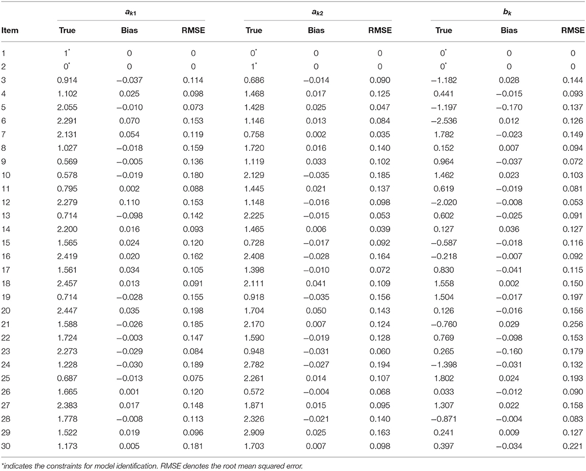
Table 3. Evaluating the accuracy of item parameter estimation.
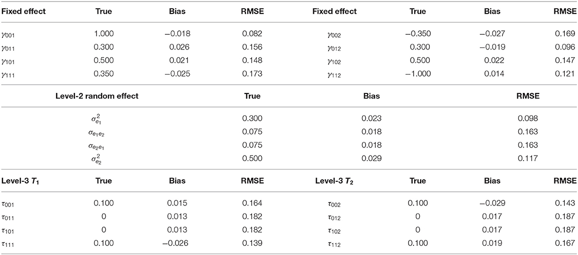
Table 4. Evaluating the accuracy of the two-dimensional fixed effects and variance-covariance components.
4.2. Simulation 2
The purpose of this simulation study is to verify whether the Gibbs sampling algorithm can guarantee the accuracy of parameters estimation when the dimensions of latent ability increase so that it can be used to guide real data analysis later. The simulation design is as follows.
The number of dimensions is fixed at 4. The multidimensional normal ogive IRT model is used to generate responses. Two factors and their varied conditions are considered: (a) number of individuals, N = 1,000, 2,000, or 3,000; (b) number of items, K = 40, 100, or 200, and for per subtest number of itmes, 10, 25, or 50. Fully crossing the different levels of these two factors yield 9 conditions. Individuals (N = 1,000, 2,000, 3,000) are equally distributed to 10 schools (J = 10). True values of item parameters and priors of all of parameters are generated by the same in simulation 1. The true values of the fixed effects are, respectively, 1.000(γ00q), 0.300(γ01q), 0.500(γ10q) and 0.350(γ11q), q = 1, 2, 3, 4, and the level-2 variance are 0.300, 0.500, 0.750, and 1.000 and the covariance are set to 0.075. The level-3 variance are 0.1 (τ00q, τ11q), and the covariance are 0 (τ01q, τ10q). The multilevel structural models (Equations 2.2 and 2.3) in simulation study 1 are used, but the dimensions are fixed at 4.
The accuracy of the parameter estimates is measured by two evaluation indexes, namely, Bias and RMSE. The recovery results are based on the MCMC iterations repeated 100 times. The detail results of the accuracy of the parameter estimates under nine conditions are display in Table 5. The Biases are −0.089~0.094 for the fixed effect parameters, −0.063~0.117 for the level-2 variance-covariance component parameters, −0.069~0.105 for the level-3 variance-covariance component parameters. The RMSEs are 0.152~0.311 for the fixed effect parameters, 0.147~0.438 for the level-2 variance-covariance component parameters, 0.132~0.382 for the level-3 variance-covariance component parameters. Furthermore, the Bias and RMSE have a smaller trend with the increase in the number of individuals and items; in other words, increasing the number of individuals and items helps to improve the estimation accuracy of the structural parameters. In summary, the Gibbs sampling algorithm is effective for various numbers of individuals and items, and it can be used to guide practices.
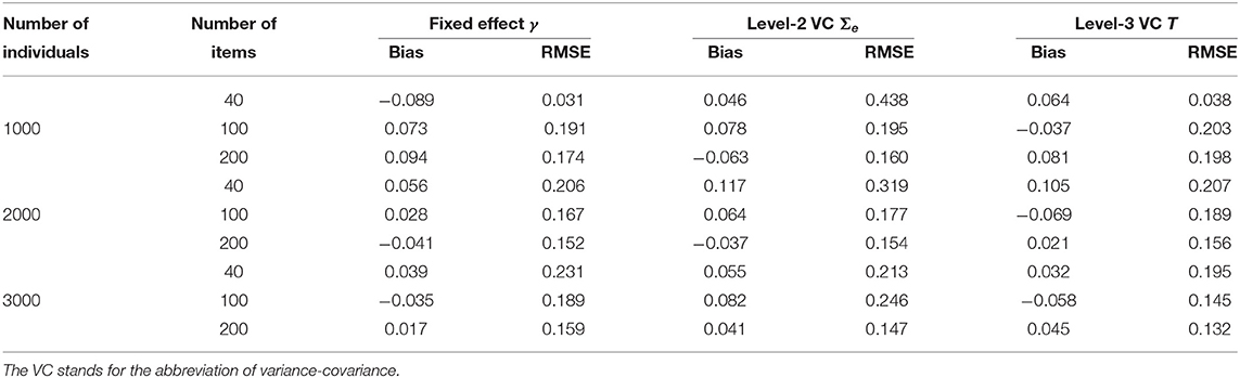
Table 5. Evaluating the accuracy of the structure parameters in the simulation 2.
5. Real Data Analysis−Examining the Correlation Between Different Ability Dimensions and Covariates
To illustrate the applicability of the multidimensional two-parameter normal ogive model in operational large-scale assessments, we consider a data set about students' English achievement test for junior middle schools conducted by NENU Branch, Collaborative Innovation Center of Assessment toward Basic Education Quality at Beijing Normal University. The analysis of the test data will help us to gain a better understanding of the practical situation of students' English academic latent traits and to explore the factors that affect their English academic latent traits. The results of this analysis will be potentially very valuable for development and improvement of educational quality monitoring mechanism in China.
5.1. Data Description
The data contain a two-stage cluster sample of 2,029 students in grade 7. These students are from 16 schools, with 121–134 students in each school. In the first stage, the sampling population is classified according to district, and schools are selected at random. In the second stage, students in grade 7 are selected at random from each school. The English test is a test battery consisting of four subscales: vocabulary (40 items), grammar (24 items), comprehensive reading (40 items), and table computing (20 items). All 124 multiple-choice items are scored using a dichotomous format. The Cronbach's alpha coefficients for vocabulary, grammar, reading comprehension and table computing items are 0.942, 0.875, 0.843, and 0.816, respectively. Level-2 and level-3 background covariates of individuals, teacher satisfaction, and school climate (teachers and schools constitute level 3) are measured. At the individual level, gender (0=male, 1=female) and socioeconomic statuses are measured; the latter is measured by the average of two indicators: the father's and mother's education, which are five-point Likert items; scores range from 0 to 8. At the teacher and school levels, teacher satisfaction is measured by 20 five-point Likert items, and school environment from the principal's perspective is measured by 23 five-point Likert items.
5.1.1. Prior Distributions
Based on the setting of priors in the simulation 1, we give the prior distributions of parameters involved in following the real data analysis. The priors of the difficulty parameters and discrimination parameters are set from bk ~ N(0, 1) and j = 1, 2, …, 124, where I4×4 is 4-by-4 identity matrix. The fixed effect γ follows a uniform distribution U(−2, 2). The prior to the variance-covariance matrix of the level-2 ability dimensions is a 4-by-4 identity matrix. The prior to the variance-covariance matrix of the level-3 T1, T2, T3, and T2 are set to non-informative priors based on Fox and Glas (2001)'s paper, where p (Tq) ∝ constant, q = 1, 2, 3, 4.
5.1.2. Convergence Diagnosis
The full conditional distribution of Gibbs sampling is run for 20,000 iterations using real data. The trace plots of parameters stabilize after 5,000 iterations. Thus, the first 5,000 iterations are set as the burn-in period. The average over the drawn parameters is calculated after the burn-in period. Moreover, Four chains started at overdispersed starting values are run for monitoring the convergence. The Brook-Gelman ratios are close to 1.2. Therefore, it can be inferred that the estimated parameters are convergent.
5.2. Model Selection in Real Data
In the real data example, we consider four dimensions of ability: vocabulary cognitive ability, grammar structure diagnosing ability, reading comprehension ability, and table computing ability. These abilities are affected by individual covariates such as socioeconomic status and gender. The individual can be nested into higher group levels (school), which are affected by group covariates such as teacher satisfactions and school climate from the teachers' perspective. In this current study, we only focus on the specific abilities of four dimensions without the general ability, which is different from Huang and Wang (2014, p. 497, Equation 3)'s ability model with hierarchical structure. According to the above-mentioned DIC model selection method, three models are considered in fitting the real data, in which the DIC can be formulated to choose between models that differ in the fixed and/or random part of the structural model to combine with the measurement model. The multidimensional IRT measurement model is identical to the three candidate models. The structural multilevel model 1 consists of the two level-2 background variables SES and Gender and the level-2 random intercept. The effects of the level-2 background variables SES and Gender are fixed across schools. The structural multilevel part is given by
Model 2 is extended by including two latent predictors at level 3, Satisfaction and Climate. The effects of the level-2 background variable SES are allowed to vary across schools. The structural multilevel part is given by
Model 3 captures the effects of the level-2 background variables SES and Gender, which are allowed to vary across schools. The structural multilevel part is given by
Question (1): According to the model selection results, which model is the best to fit the data and how can judge the individual-level regression coefficients be judged as fixed effect or random effect?
The estimated DIC values are presented in Table 6. Model 2 shows that the smallest effective number of model parameters among the three models, which is preferred given the DIC values of the three models. The DIC values of models 2 and 3 are smaller than those of model 1, which can be attributed to the additional latent predictors at level 3, i.e., Satisfaction and Climate. Note that in model 2, the individual random-effect parameters are modeled as group-specific random effects (level-3 Satisfaction and Climate latent predictors), leading to a serious reduction in the effective number of model parameters, which can be inferred from the PD value in Table 6. The DIC value of model 2 is smaller than that of model 3. The residual u2jq of the random effect β2jq is estimated equal to 0, which is equivalent to fixing the effect of the level-2 background variable Gender across schools.
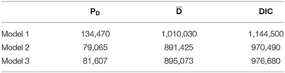
Table 6. Estimated DIC values for the three models fitted to the English test data.
5.3. Structural Parameter Analysis
Over the past 40 years, a large number of studies have shown that there is a direct relationship between the individuals' language learning ability and the parents' education. For example, Teachman (1987) made use of high school survey data in the United States to explore the influence of family background on childhood education. The results of this study indicated that the parents' occupations, incomes, and educations have a very important impact on children language academic achievement. Moreover, Stern (1983) shows that language is a social mechanism, which needs to be learned in the social environment, even in the biological basis play an important role of mother tongue acquisition, social factors related to children and their parents also play an important role. However, in our study, whether the parents' educational level (SES) has influence on the four kinds of abilities in English learning; the following question will be considered:
Question (2): How will students from different ends of the socioeconomic-status (SES) score in English performance as tested in four types of latent abilities, based on the level-2 gender (GD), level-3 teacher satisfaction (ST) and school climate (CT).
From Tables 7–10, we can find that the estimated fixed effects γ10q(SES) are 0.642, 0.312, 0.542, and 0.596 for q = 1, 2, 3, 4, respectively. It can be observed that students with high SES scores perform better than students with low SES scores, where performance is measured by four types of latent abilities when controlling for the level-2 GD individual covariates and the level-3 ST and CT school covariates. That is, their parents' educational level differs by one unit for the male students from the same class and school. In English learning, vocabulary cognitive ability, the ability to diagnose grammar structure, reading comprehension ability and table computing ability have the differences of 0.642, 0312, 0.542, and 0.596, respectively. The rate of increase in grammatical diagnostic ability (0.312) is markedly smaller than that of the other three kinds of abilities. In addition, compared to male students, the differences in the four dimensions of ability are 0.981, 0.706, 0.874, and 0.330 for female students, respectively. In summary, the education of parents (SES) is responsible for students' English learning abilities. The parents with a high SES values have more prospective awareness in English learning based on their own learning experiences, provide more diversified learning ways, and know how to create a better English learning environment for students. In addition, parents with better education can provide more important learning guidance in English. In general, the better the parents' education, the better they will able to tutor student's English learning.
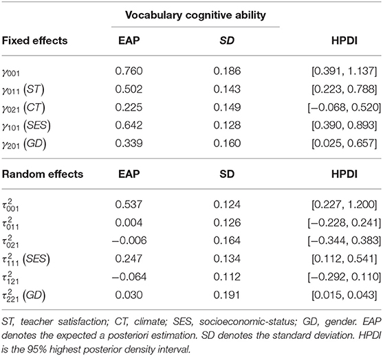
Table 7. Parameter estimation of the multilevel multidimensional IRT model for vocabulary cognitive ability.

Table 8. Parameter estimation of the multilevel multidimensional IRT model for diagnosing ability of grammar structure.
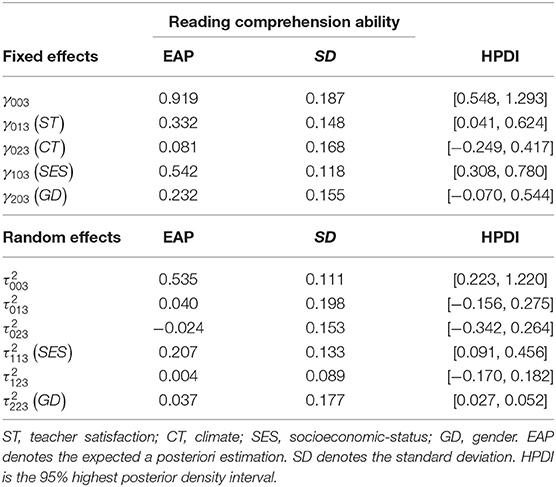
Table 9. Parameter estimation of the multilevel multidimensional IRT model for reading comprehension ability.
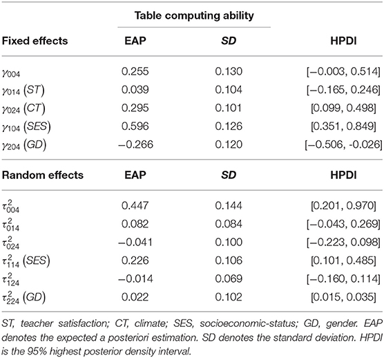
Table 10. Parameter estimation of the multilevel multidimensional IRT model for table computing ability.
Etaugh and Bridges (2003), Li (2005), and Burstall (1975) found that females were better than males in most of the language tasks (vocabulary, reading, grammar, spelling and writing), and the difference in language ability appeared earlier than other cognitive abilities. In infancy, females show more linguistic advantages than males, and they speak more fluently, and have a richer vocabulary. To about 11 years old, they are not only good at simple spelling, but also are able to do more complicated writing tasks. In schools, teachers have found that females do better in reading comprehension, and they are less likely to have reading problems, including reading barriers. However, whether or not have the above conclusions in this study, next the following issues will be considered:
Question (3): What relationship exists between males and females' performances in different latent abilities by controlling for SES, ST and CT?
Results from Tables 7–10 show that for male and female students from the same class and school with the same SES scores, female students' performances of vocabulary cognitive ability, the ability to diagnose grammar structure and reading comprehension ability are higher than those of male students 0.339, 0.394, 0.232. However, male students have a 0.266 advantage over female students in table computing ability. This empirical study yields almost identical conclusions for Etaugh and Bridges (2003). That is, male and female students, who have the same SES scores in the same class and school, have a great difference in the acquisition of English proficiency. Moreover, in terms of vocabulary cognition, grammatical structure analysis, reading comprehension it can be seen that females are better than males at vivid memory and mechanical memory is stronger than males. However, compared to females, males are markedly better than females at logical reasoning, deductive induction, and computing ability. In addition, according to gender difference in English learning of middle school students, the improving measure of learning from others' strong points to offset one' own weakness mainly covers: first, either teachers of students should properly understand the gender difference; second, to strengthen female students' training of logical thinking; third, to widen female students' reasoning computing ability; fourth, for the male students, to develop their vivid memory through a variety of teaching methods. These four points should be parallel in structure.
Question (4): What effects, if any, are seen with different teachers' or schools' effects (covariates)?
For male students who have the same SES scores from different schools, if the difference in teacher satisfaction is a unit, the difference in vocabulary cognitive ability, the ability to diagnose grammar structure and reading comprehension ability are 0.502, 0.335, and 0.331, respectively. However, the difference in the table computing ability is very small for 0.039. Teachers' factor has an important effect on students' cognitive ability, the ability to diagnose grammar structure and reading ability. On the contrary, the table computing ability has little impact.
This study indicates that the middle school teachers with high teacher satisfactions have a strong sense of responsibility, can be filled with enthusiasm in the work of education and teaching, and inspire students' learning motivation. This results in a great improvement in the students' vocabulary cognitive ability, the ability to analyze grammatical structure and reading comprehension ability owing to teachers' teaching attitude and responsibility. However, the margin of the improvement for the table computing ability is small. It is possible to play a decisive role in the students' internal factors as compared with the teachers' external factors.
As we know, people are the product of the environment. The environment has a great impact on cognition, emotion and behavior intention. Different people live in different environments so that there is a huge difference in cognition, emotion and behavior intention. Similarly, in English teaching, are whether or not the performances identical for different schools' effects (school climate)? If not, what are the effects?
The estimated results for school climate effects γ02q are 0.225, 0.081, 0.086, and 0.295 for q = 1, 2, 3, 4, respectively. The performances associated with vocabulary cognitive ability and table computing ability are markedly affected by the level-3 CT covariates, whereas the ability to diagnose grammar structure and reading comprehension ability are not markedly affected when controlling for the level-2 SES and GD individual covariates and the level-3 ST school covariates. Analysis of the level-3 variance components reveals that the values of (SES) are markedly different from 0, and their estimates are 0.247, 0.272, 0.207, and 0.226 for q = 1, 2, 3, 4, respectively. This result illustrates that the effect of SES varies from school to school. In addition, the (GD) values are not markedly different from 0. In addition, according to the DIC model selection results, model 2 shows the best fit to the real data when β2jq are defined as fixed effects. The estimation results show that the proportion of females to males does not vary among schools. The estimation covariance between the random effects , , and are all not markedly different from 0. It can be concluded that the random effects are independent of each other for each type of ability. All estimated parameters are shown in Tables 7–10.
5.4. Item Test Dimension Evaluation
Question (5): Is it possible to use a measurement tool to determine whether items' factor patterns correlate to the subscales of the test battery? In particular, will the four subtests of the test battery be discernable according to the discrimination parameters on the four dimensions?
A test battery contains four subtests, which consist of items of measuring four dimensional abilities, and a type of latent ability can be measured mainly by a subtest. It can be observed that the EAP estimates of the discrimination parameters are plotted to determine whether the items' factor patterns reflect the subtest of the test battery in Figure 1. In the left-hand panel of Figure 1, the discrimination parameters of the first two dimensions are plotted for subtest 1 (items marked by a dot) and subtest 2 (items marked by a star), and the other items are marked by a diamond. It can be observed that the items of subtest 1 (1–40 item) have a high factor loading on the first dimension and a low factor loading on the second dimension, and the items of subtest 2 (41–64 item) have a high factor loading on the second dimension and a low factor loading on the first dimension. The other items do not vary appreciably between the two dimensions. The right-hand panel of Figure 1 shows the pattern of the discrimination parameters of the third and fourth subtests on the third and fourth dimensions. The items of subtest 3 (65–104 item) have a high factor loading on the third dimension and a low factor loading on the fourth dimension, and the items of subtest 4 (105–124 item) have a high factor loading on the fourth dimension and a low factor loading on the third dimension. The overall pattern of the discrimination parameters fit the test battery quite well, demonstrating that each dimension is identified by items of one subtest.
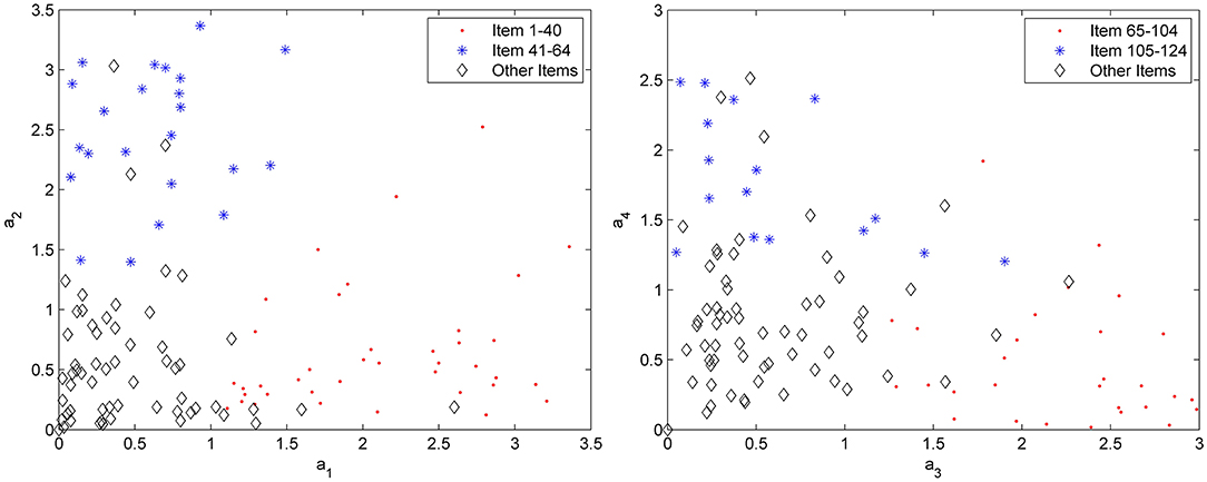
Figure 1. Parameters of estimation ak1, ak2, ak3, and ak4 for subscale 1 (items 1–40), subscale 2 (items 41–64), subscale 3 (items 65–104), and subscale 4 (items 105–124).
6. Concluding Remarks
In this study, we mainly focus on constructing a multilevel multidimensional model to fit the hierarchical dataset about a large-scale English achievement test. Particular attention is given to assessing the correlation between multiple latent abilities and covariates.
In view of the characteristics of the test structure (i.e., (1) the students are nested within classes or schools; (2) the binary response consists of several subtests and each subtest measures a distinct latent trait), we extend the measurement model developed by Fox and Glas (2001) and Kamata (2001) to the multidimensional case by replacing their unidimensional IRT model with a multidimensional normal ogive model. The numerical results show that the multidimensional IRT model is appropriate for modeling the measurement model. It can accurately model the item/person interaction and utilize the correlations between subtests to increase the measurement precision of each subtest.
From what has been using the above empirical data, we may safely draw valuable conclusions to provide guidance for the future English teaching. Socioeconomic status (SES) has a positive impact on the abilities of four dimensions. That is, the higher families' SESs, the better performances in the four dimensional abilities. In addition, the study also found that students of different genders do not demonstrate the same level of expertise in English skills are expert in the English skills are not the same. Female students are good at the items related to the memory of the image and mechanical memory, such as the vocabulary, grammar and reading comprehension; but the male students have the advantage in reasoning calculation. Therefore, teachers should adjust the teaching methods based on the gender differences so that he or she can acquire the ability to overcome their own deficiency. Teachers' satisfaction as level 3 teacher covariate markedly impacts English table computing ability. It is possible to play a decisive role in the students' internal factors as compared with the teachers' external factors. Finally, the impact of the school climate factor on students' grammatical structure analysis and reading comprehension is not very obvious, and the specific reasons are to be studied later.
In the future studies, the correlations between schools at the level-3 should be taken into consideration. For example, the different secondary schools which are located in the same district may share a common education resources. In addition, the measurement model can be improved by considering polytomous item response theory model to analyze ordinal response data with more information. As an extension of this paper, the polytomous response model associated with the multilevel models can be used to help evaluate the multiple latent abilities, which may be more suitable for the current complex situation of educational and psychological research. In the field of estimation method, Bayesian estimation method will face serious challenges when the number of examinees or the number of items, or MCMC sample size are substantially increased. Therefore, the proposal of efficient Bayesian algorithm and the development of easy-to-use software package are also important research focus in the later period.
Data Availability Statement
The datasets for this manuscript are not publicly available because Data from NENU Branch, Collaborative Innovation Center of Assessment toward Basic Education Quality at Beijing Normal University has signed a confidentiality agreement. Requests to access the datasets should be directed todGFvakBuZW51LmVkdS5jbg==.
Author Contributions
FC completed the writing of the article. JL and JT provided key technical support. JZ provided original thoughts and article revisions.
Funding
This research was supported by the National Natural Science Foundation of China (Grant 11571069).
Conflict of Interest
The authors declare that the research was conducted in the absence of any commercial or financial relationships that could be construed as a potential conflict of interest.
Acknowledgments
We would like to thank the Editor, and two referees for their constructive suggestions and comments, which have led to an improved version of the manuscript.
Supplementary Material
The Supplementary Material for this article can be found online at: https://www.frontiersin.org/articles/10.3389/fpsyg.2019.02387/full#supplementary-material
Figure S1. Trace plot of a9,1.
Figure S2. Trace plot of a9,2.
Figure S3. Trace plot of b9.
Figure S4. Trace plot of a26,1.
Figure S5. Trace plot of a26,2.
Figure S6. Trace plot of b26.
Figure S7. Trace plots of the fixed effects in the first dimension.
Figure S8. Trace plots of the fixed effects in the second dimension.
Figure S9. Trace plot of .
Figure S10. Trace plot of σe1e2.
Figure S11. Trace plot of .
Figure S12. Trace plot of τ001.
Figure S13. Trace plot of τ002.
Figure S14. Trace plot of τ011τ101.
Figure S15. Trace plot of τ012τ102.
References
Ackerman, T. A. (1989). Unidimensional IRT calibration of compensatory and noncompensatory multidimensional items. Appl. Psychol. Meas. 13, 113–127. doi: 10.1177/014662168901300201
Adams, R. J., Wilson, M., and Wu, M. (1997). Multilevel item response models: an approach to errors in variables regression. J. Educ. Behav. Stat. 22, 47–76. doi: 10.3102/10769986022001047
Albert, J. H. (1992). Bayesian estimation of normal ogive item response curves using Gibb ssampling. J. Educ. Stat. 17, 251–269. doi: 10.3102/10769986017003251
Asparouhov, T., and Muthén, B. (2012). General Random Effect Latent Variable Modeling: Random Subjects, Items, Contexts, and Parameters. Available online at: https://www.statmodel.com/download/NCME12.pdf
Béguin, A. A., and Glas, C. A. W. (2001). MCMC estimation of multidimensional IRT models. Psychometrika 66, 541–561. doi: 10.1007/BF02296195
Bock, R. D., and Aitkin, M. (1981). Marginal maximum likelihood estimation of item parameters: application of an EM algorithm. Psychometrika 46, 443–459. doi: 10.1007/BF02293801
Bock, R. D., and Schilling, S. G. (2003). “IRT based item factor analysis,” in IRT from SSI: BILOG-MG, MULTILOG, PARSCALE, TESTFACT, ed M. du Toit (Lincolnwood, IL: Scientific Software International), 584–591.
Box, G. E. P., and Tiao, G. C. (1973). Bayesian Inference in Statistical Analysis. Reading, MA: Addison-Wesley.
Bradlow, E. T., Wainer, H., and Wang, X. (1999). A Bayesian random effects model for testlets. Psychometrika 64, 153–168. doi: 10.1007/BF02294533
Brooks, S. P., and Gelman, A. (1998). Alternative methods for monitoring convergence of iterative simulations. J. Comput. Graph. Stat. 7, 434–455. doi: 10.1080/10618600.1998.10474787
Burstall (1975). Factors affecting foreign language learning: a consideration of some recent research findings. Lang. Teach. Linguist. Abstr. 29, 132–140. doi: 10.1017/S0261444800002585
Cai, L. (2010a). High-dimensional exploratory item factor analysis by a Metropolis-Hastings Robbins-Monro algorithm. Psychometrika 75, 33–57. doi: 10.1007/s11336-009-9136-x
Cai, L. (2010b). Metropolis-Hastings Robbins-Monro algorithm for confirmatory item factor analysis. J. Educ. Behav. Stat. 35, 307–335. doi: 10.3102/1076998609353115
Cai, L. (2010c). A two-tier full-information item factor analysis model with applications. Psychometrika 75, 33–57. doi: 10.1007/s11336-010-9178-0
Cai, L. (2013). flexMIRT: Flexible Multilevel Multidimensional Item Analysis and Test Scoring (Version 2) [Computer software]. Chapel Hill, NC: Vector Psychometric Group.
Chalmers, R. P. (2015). Extended mixed-effects item response models with the MH-RM algorithm. J. Educ. Meas. 52, 200–222. doi: 10.1111/jedm.12072
De Jong, M. G., and Steenkamp, J. B. E. M. (2010). Finite mixture multilevel multidimensional ordinal IRT models for large scale cross-cultural research. Psychometrika 75, 3–32. doi: 10.1007/s11336-009-9134-z
Embretson, S. E., and Reise, S. P. (2000). Item Response Theory for Psychologists. Mahwah, NJ: Lawrence Erlbaum.
Etaugh, C., and Bridges, J. S. (2003). The Psychology of Women: A Lifespan Perspective. Boston, MA: Allyn & Bacon.
Fox, J. P., and Glas, C. A. W. (2001). Bayesian estimation of a multilevel IRT model using Gibbs sampling. Psychometrika 66, 271–288. doi: 10.1007/BF02294839
Fraser, C. (1988). NOHARM: A Computer Program for Fitting Both Unidimensional and Multidimensional Normal Ogive Models of Latent Trait Theory. Armidale, NSW: University of New England.
Gelman, A., Carlin, J. B., Stern, H. S., Dunson, D. B., Vehtari, A., and Rubin, D. B. (2014). Bayesian Data Analysis, 3rd Edn. Boca Raton, FL: CRC Press.
Gelman, A., Meng, X. -L., and Stern, H. S. (1996). Posterior predictive assessment of model fitness via realized discrepancies. Stat. Sin. 6, 733–807.
Geman, S., and Geman, D. (1984). Stochastic relaxation, Gibbs distribution and the Bayesian restoration of images. IEEE Trans. Pattern Anal. Machine Intell. 6, 721–741. doi: 10.1109/tpami.1984.4767596
Höhler, J., Hartig, J., and Goldhammer, F. (2010). Modeling the multidimensional structure of students' foreign language competence within and between classrooms. Psychol. Test Assess. Model. 52, 323–340. Retrieved from: http://www.psychologie-aktuell.com/fileadmin/download/ptam/3-2010_20100928/07_Hoehler.pdf
Holtmann, J., Koch, T., Lochner, K., and Eid, M. (2016). A comparison of ml, wlsmv, and bayesian methods for multilevel structural equation models in small samples: a simulation study. Multivar. Behav. Res. 51, 661–680. doi: 10.1080/00273171.2016.1208074
Hox, J. (2002). Multilevel Analysis, Techniques and Applications. New Jersey: Lawrence Erlbaum Associates.
Huang, H.-Y., and Wang, W.-C. (2014). Multilevel higher-order item response theory models. Educ. Psychol. Meas. 73, 495–515. doi: 10.1177/0013164413509628
Huang, H.-Y., Wang, W.-C., Chen, P.-H., and Su, C.-M. (2013). Higher-order item response theory models for hierarchical latent traits. Appl. Psychol. Meas. 37, 619–637. doi: 10.1177/0146621613488819
Kamata, A. (2001). Item analysis by the hierarchical generalized linear model. J. Educ. Meas. 38, 79–93. doi: 10.1111/j.1745-3984.2001.tb01117.x
Kelderman, H., and Rijkes, C. P. M. (1994). Loglinear multidimensional IRT models for polytomously scored items. Psychometrika 59, 149–176. doi: 10.1007/BF02295181
Kim, S. (2001). An evaluation of the Markov chain Monte Carlo method for the Rasch model. Appl. Psychol. Meas. 25, 163–176. doi: 10.1177/01466210122031984
Klein Entink, R. H. (2009). Statistical models for responses and response times (Ph.D. dissertation). University of Twente, Faculty of Behavioural Sciences, Enschede, Netherlands.
Klein Entink, R. H., Fox, J. P., and van der Linden, W. J. (2009). A multivariate multilevel approach to the modeling of accuracy and speed of test takers. Psychometrika 74, 21–48. doi: 10.1007/s11336-008-9075-y
Li, L. J. (2005). A Study on Gender Differences and Influencing Factors of High School Students' English Learning. Fuzhou: Fujian Normal University Press.
Lindley, D. V., and Smith, A. F. M. (1972). Bayes estimates for the linear model. J. R. Stat. Soc. B 34, 1–41. doi: 10.2307/2985048
Lu, I. R., Thomas, D. R., and Zumbo, B. D. (2005). Embedding IRT in structural equation models: a comparison with regression based on IRT scores. Struct. Equat. Model. 12, 263–277. doi: 10.1207/s15328007sem1202_5
Lu, Y. (2012). A multilevel multidimensional item response theory model to address the role of response style on measurement of attitudes in PISA 2006. (Doctoral dissertation). University of Wisconsin, Madison, WI, United States, 164.
Mulaik, S. A. (1972). “A mathematical investigation of some multidimensional rasch models for psychological tests,” in Paper Presented at the Annual Meeting of the Psychometric Society (Princeton, NJ).
Muraki, E., and Carlson, J. E. (1993). “Full-information factor analysis for polytomous item responses,” in Paper Presented at the Annual Meeting of the American Educational Research Association (Atlanta, GA).
Muthén, B. O., and Asparouhov, T. (2013). “Item response modeling in Mplus: a multi-dimensional, multi-level, and multi-time point example,” in Handbook of Item Response Theory: Models, Statistical Tools, and Applications. Retrieved from: http://www.statmodel.com/download/IRT1Version2.pdf
Muthén, B. O., du Toit, S. H. C., and Spisic, D. (1997). Robust Inference Using Weighted Least Squares and Quadratic Estimating Equations in Latent Variable Modeling With Categorical and Continuous Outcomes. Unpublished technical report.
Muthén, L. K., and Muthén, B. O. (1998). (1998–2012). Mplus User's Guide, 7th Edn. Los Angeles, CA: Muthén & Muthén.
Pastor, D. A. (2003). The use of multilevel IRT modeling in applied research: an illustration. Appl. Meas. Educ. 16, 223–243. doi: 10.1207/S15324818AME1603_4
Patz, R. J., and Junker, B. W. (1999a). A straightforward approach to Markov chain Monte Carlo methods for item response models. J. Educ. Behav. Stat. 24, 146–178. doi: 10.3102/10769986024002146
Patz, R. J., and Junker, B. W. (1999b). Applications and extensions of MCMC in IRT: multiple item types, missing data, and rated responses. J. Educ. Behav. Stat. 24, 342–366. doi: 10.3102/10769986024004342
Plummer, M. (2003). “JAGS: a program for analysis of Bayesian graphical models using Gibbs sampling,” in Proceedings of the 3rd International Workshop on Distributed Statistical Computing, eds K. Hornik, F. Leisch, and A. Zeileis (Vienna). Available online at: http://www.ci.tuwien.ac.at/Conferences/DSC-2003/Proceedings/
Reckase, M. D. (1972). Development and application of a multivariate logistic latent trait model. (Unpublished doctoral dissertation). Syracuse University, Syracuse, NY, United States.
Reckase, M. D. (2009). Multidimensional Item Response Theory. New York, NY: Springer Science Business Media, LLC.
Rupp, A. A., Dey, D. K., and Zumbo, B. D. (2004). To Bayes or not to Bayes, from whether to when: applications of Bayesian methodology to modeling. Struct. Equat. Model. 11, 424–451. doi: 10.1207/s15328007sem1103_7
Samejima, F. (1974). Normal ogive model on the continuous response level in the multidimensional space. Psychometrika 39, 111–121. doi: 10.1007/BF02291580
Shalabi, F. (2002). Effective schooling in the west bank (Ph.D. dissertation). University of Twente, Enschede, Netherlands.
Sheng, Y. (2010). A sensitivity analysis of Gibbs sampling for 3PNO IRT models: effects of prior specifications on parameter es timates. Behaviormetrika 37, 87–110. doi: 10.2333/bhmk.37.87
Sheng, Y., and Wikle, C. K. (2007). Bayesian multidimensional IRT models with a hierarchical structure. Educ. Psychol. Meas. 68, 413–430. doi: 10.1177/0013164407308512
Skrondal, A., and Rabe-Hesketh, S. (2004). Generalized Latent Variable Modeling: Multilevel, Longitudinal and Structural Equation Models. Boca Raton, FL: Chapman & Hall.
Song, X.-Y., and Lee, S.-Y. (2012). A tutorial on the Bayesian approach for analyzing structural equation models. J. Math. Psychol. 56, 135–148. doi: 10.1016/j.jmp.2012.02.001
Spiegelhalter, D. J, Thomas, A., Best, N. G., and Lunn, D. (2003). WinBUGS Version 1.4 User Manual. Cambridge: MRC Biostatistics Unit. Available online at: http://www.mrc-bsu.cam.ac.uk/bugs/
Spiegelhalter, D. J., Best, N. G., Carlin, B. P., and Linde, A. V. D. (2002). Bayesian measures of model complexity and fit. J. R. Stat. Soc. Ser. B 64, 583–639. doi: 10.1111/1467-9868.00353
Sympson, J. B. (1978). “A model for testing with multidimensional items,” in Proceedings of the 1977 Computerized Adaptive Testing Conference, ed D. J. Weiss (Minneapolis, MN: University of Minnesota).
Tanner, M. A., and Wong, W. H. (1987). The calculation of posterior distributions by data augmentation. J. Am. Stat. Assoc. 82, 528–550. doi: 10.1080/01621459.1987.10478458
Teachman, J. D. (1987). Family background, educational resources, and educational attainment. Am. Sociol. Rev. 52, 548–557. doi: 10.2307/2095300
van der Linden, W. J. (2007). A hierarchical framework for modeling speed and accuracy. Psychometrika 72, 287–308. doi: 10.1007/s11336-006-1478-z
van der Linden, W. J. (2008). Using response times for item selection in adaptive testing. J. Educ. Behav. Stat. 33, 5–20. doi: 10.3102/1076998607302626
Wang, C., Xu, G., and Shang, Z. (2018). A two-stage approach to differentiating normal and aberrant behavior in computer based testing. Psychometrika 83, 223–254. doi: 10.1007/s11336-016-9525-x
Way, W. D., Ansley, T. N., and Forsyth, R. A. (1988). The comparative effects of compensatory and non-compensatory two-dimensional data on unidimensional IRT estimates. Appl. Psychol. Meas. 12, 239–252. doi: 10.1177/014662168801200303
Whitely, S. E. (1980a). Measuring Aptitude Processes With Mutlicomponent Latent Trait Models. Technical Report No. NIE-80-5. Lawrence, KS: University of Kansas.
Whitely, S. E. (1980b). Multicomponent latent trait models for ability tests. Psychometrika 45, 479–494. doi: 10.1007/BF02293610
Yao, L., and Schwarz, R. (2006). A multidimensional partial credit model with associated item and test statistics: an application to mixed-format tests. Appl. Psychol. Meas. 30, 469–492. doi: 10.1177/0146621605284537
Keywords: education assessment, teacher satisfactions, multidimensional item response theory, multilevel model, Bayesian estimation
Citation: Zhang J, Lu J, Chen F and Tao J (2019) Exploring the Correlation Between Multiple Latent Variables and Covariates in Hierarchical Data Based on the Multilevel Multidimensional IRT Model. Front. Psychol. 10:2387. doi: 10.3389/fpsyg.2019.02387
Received: 25 April 2019; Accepted: 07 October 2019;
Published: 25 October 2019.
Edited by:
Jason C. Immekus, University of Louisville, United StatesReviewed by:
Peida Zhan, Zhejiang Normal University, ChinaYong Luo, Educational Testing Service, United States
Copyright © 2019 Zhang, Lu, Chen and Tao. This is an open-access article distributed under the terms of the Creative Commons Attribution License (CC BY). The use, distribution or reproduction in other forums is permitted, provided the original author(s) and the copyright owner(s) are credited and that the original publication in this journal is cited, in accordance with accepted academic practice. No use, distribution or reproduction is permitted which does not comply with these terms.
*Correspondence: Jiwei Zhang, emhhbmdqdzcxM0BuZW51LmVkdS5jbg==