Passive evaporative coolers for postharvest storage of fruit and vegetables: Where to best deploy them and how well do they perform

Passive evaporative coolers have a huge potential to help smallholder farmers to preserve their fresh fruit and vegetables longer after harvest. However, we could benefit from more transparent information on where evaporative coolers perform sufficiently well to extend the postharvest life of the fresh produce significantly. Unsatisfactory evaporative cooler performance is a potential cause for farmers' limited adoption of this technology to reduce food losses. Our objective is to present easy-to-use tools that help to better scope regions with the best potential for direct passive evaporative coolers and for effectively deploying it. This information should help avoid installing evaporative coolers in areas with environmental conditions that only induce a temperature depression of a few degrees Celsius. Concretely, we developed design charts of the achievable temperature depression by evaporative cooling based on the local air temperature and humidity. We quantified for apple, banana, mango, and tomato the resulting additional days in postharvest life gained by storing the produce in an evaporative cooler. For these fruits, the gain in postharvest life using passive cooling is roughly 2–15 days for temperate climates with an ambient temperature of 20°C and a humidity of 50%. We present geographical maps of India, Nigeria, and the entire world at a 30 km resolution that answer how much evaporative cooling can maximally decrease the produce temperature and extend postharvest life for banana fruit. We found that passive evaporative cooling could induce up to a 7-day gain in postharvest life. We make these maps available online. We also quantify how well evaporative coolers perform concerning reducing the temperature and how they should be sized. Our results will facilitate installing evaporative coolers only in suitable regions. Our data also show in which months the cooler can be operated with the best performance. We thereby help avoid disillusion and loss of trust in the technology with smallholder farmers, policymakers, farmers, or farmer cooperatives. Further catalyzing the implementation of small-scale evaporative coolers can bring farmers significant gains in postharvest life, reduce food losses, and increase revenues.

1 Introduction

Evaporative cooling is a high-potential technological innovation that can help preserve fresh foods (GKI, 2017; Verploegen, 2021a). Evaporative coolers extract heat from the surrounding air and the fruit or vegetables in the cooler. This heat is the latent heat required to evaporate water. This water is absorbed by the porous material inside the cooler (e.g., charcoal). In such evaporative coolers, we can reduce the product’s temperature by typically 3°C–10°C and increase the relative humidity inside the cooler to up to 70%–100% (Defraeye et al., 2022). The reduced rate of food deterioration at lower temperatures and the reduced moisture loss help preserve the fruit or vegetables longer. Evaporative coolers work best in dry and warm regions.

These passive cooling systems are especially interesting for marginal or smallholder farmers and single-family households in remote, off-grid areas (Elansari et al., 2019; Teutsch and Kitinoja, 2019). If they are not part of a larger cooperative or farmer-producer organization (FPO), these stakeholders do not always have access to active cooling or cannot afford it. Nevertheless, smallholder farmers produce a large amount of the world’s food. Increased smallholder productivity is thus a large growth driver in future postharvest supply chains (Ricciardi et al., 2018; Boettiger and Sanghvi, 2019; Goedde et al., 2019). We would benefit of affordable cooling solutions for smallholder farmers, one of which could be evaporative cooling. Evaporative cooling is also argued to be one of the key investable innovations for emerging markets that can transform these food systems (GKI, 2017; Verploegen, 2021a). Such a solution is implementable with limited training and acceptable capital costs.

Several types of evaporative cooling systems are known. Examples are the zeer pot, sand and brick coolers, khus-mat coolers, and charcoal coolers (Elansari et al., 2019; Teutsch and Kitinoja, 2019). Cooler types are direct evaporative coolers and indirect evaporative coolers. The indirect coolers just reduce the air temperature without increasing the humidity of the air. Direct evaporative coolers cool the air that is directly in contact with the fresh produce, and thereby also humidify the air. Active and passive cooler types exist, where active coolers apply forced airflow generation to evaporate water from a cooling medium. A lot of work has already been done on evaporative cooling (Anyanwu, 2004; Mittal et al., 2006; Dadhich et al., 2008; Getinet et al., 2008; Vanndy et al., 2008; Olosunde et al., 2016; Olosunde et al., 2009; Chinenye, 2011; Mogaji and Fapetu, 2011; Shitanda et al., 2011; Manuwa and Odey, 2012; Chinenye et al., 2013; Mogaji et al., 2013; Samira et al., 2013; Deoraj et al., 2015; Ogbuagu et al., 2016; Zakari et al., 2016; Alam et al., 2017; Ambuko et al., 2017; Korir et al., 2017; Poku et al., 2017; Nkolisa et al., 2018; Adekanye et al., 2019; Sibanda and Workneh, 2019; Abaranji et al., 2021; Patel et al., 2021; Raza et al., 2021; Sibanda and Seyoum Workneh, 2021). Based on this literature, postharvest storage us usually done using active (∼50%) and passive (∼30%) direct coolers. Indirect coolers make up for the remaining 20%. Direct passive evaporative coolers are used by smallholder farmers in developing countries and are the focus of this study. Such passive coolers typically store about 0.01–10 m³ of fresh produce. Water is stored in a porous material, namely a cooling pad or material. Cooling pads are typically 0.01 m–0.2 m thick. Passive coolers have been used to preserve coriander leaves, fenugreek leaves, spinach, tomato, green onion, carrot, radish, peas, papaya, sapota, orange, plum, and grapes (Dadhich et al., 2008). Previous research showed that the shelf life could be augmented by 2–6 days using an evaporative cooling system. Direct passive coolers reduced the mass loss of tomato, carrots, papaya, orange, and amaranth by up to 90%, concerning storage at ambient conditions (Dadhich et al., 2008; Ambuko et al., 2017).

Despite their potential, these coolers are not widely deployed (Kanali et al., 2017). There are several reasons for this. A problem for smallholder farmers to deploy these coolers is one of scale (Verploegen, 2021b; Defraeye et al., 2022). There are too many farmers and limited resources to have direct access to expertise, training, and sufficient capital to efficiently build and operate evaporative coolers. There is also little economic incentive for companies to produce and disseminate such small-scale cooling facilities, despite the huge potential of this technology to help preserve food worldwide. In this case, one would need to interact with and train hundreds of farmers individually. Instead, companies that provide cooling solutions are more inclined to engage with larger clusters of farmers. Engaging with only a few contact persons instead of a few hundred is more practical. Companies also prefer providing more controllable cooling solutions, such as micro-scale solar-powered cool rooms. As a result of these hurdles, we notice that scientific funding, projects, and publications in this field are also limited. Only a few institutes actively research this topic. The scientific studies that were done in developing countries are mostly very applied.

As a result of this limited scientific and economic interest, the scientific basis of evaporative cooling devices is also rather limited (Rehman et al., 2020). An in-depth understanding of the underlying processes of how evaporative coolers work and perform for postharvest applications is rarely analyzed. Information on where evaporative coolers perform best is also scarce (Verploegen, 2021b; Verploegen, 2021c). This lack of information for the stakeholders leaves key questions unanswered and hides the potential for optimization. Evaporative coolers should work to the best of their potential to (1) preserve the fresh produce as long as necessary and (2) for the farmers to keep their trust in these systems. Only then will farmers continue to use them over several seasons.

In this paper, we use the theory of evaporative cooling to answer practical questions on evaporative cooling and its application. We focus on direct passive evaporative coolers. Our objective of this work is to develop easy-to-use tools that help to more-effectively deploy direct passive evaporative coolers. We quantify the maximal temperature reduction gained by evaporative cooling and visualize it into design charts for different stakeholders. To our knowledge, such charts are not available, but they depict the interdependencies of different parameters. Additionally, we determine the possible gains in postharvest life achieved by evaporative cooling. We focus on fruits, but the findings are also relevant to vegetables. We show on a world map in which location it makes the most sense to apply evaporative cooling. Here we show the maximal temperature reduction that can be achieved. Currently, the theory is known to evaluate the performance of passive evaporative coolers, but this information has not been analyzed to our knowledge for different fruits worldwide at a resolution of 30 km. Furthermore, we quantify how much fruit we can cool with a certain amount of water. Finally, we quantify the optimal thickness of the evaporative cooler walls and how this thickness affects the cooler performance.

2 Materials and methods

2.1 Wet-bulb temperature and temperature depression calculation

We quantified the temperature depression that can be achieved by evaporative cooling. There exist many empirical equations to directly calculate the wet-bulb temperature (θ_wb [°C] or T_wb [K]) from the dry-bulb temperature (θ_db [°C] or T_db [K]) and the relative humidity of the moist air (φ_a [%]) (Stull, 2011). However, we introduced an error in predicting the wet-bulb temperature with most empirical equations. This error can amount to 0.3°C–0.6°C (see Supplementary Material). Therefore, these 'direct' equations do not provide adequate sensitivity for estimating the design parameters of an evaporative cooler. In the present study, we calculated T_wb from T_db, and φ_a using an iterative approach. This approach was based on the psychrometric constant γ [K⁻¹], which is often used to construct psychrometric tables (Jensen et al., 1990; Simões-Moreira, 1999; Allen et al., 2005). This approach converted the temperature depression (T_wb-T_db) into a vapor pressure deficit (p_v,sat(T_wb) - p_v,a(T_db)) through well-established empirical coefficients for estimating vapor pressure from temperature and quantifying the latent energy (Sadeghi et al., 2013).

$p_v〈T_{db}〉-p_{v,sat}〈T_{wb}〈T_{db},{\phi }_a〉〉+\gamma {\mathrm{P}}_{\mathrm{a}\mathrm{t}\mathrm{m}}\left(T_{db}-T_{wb}\right)=0(1)$

Here, p_v is the ambient vapor pressure at the dry-bulb temperature [Pa], p_v,sat is the saturated vapor pressure [Pa] at the wet-bulb temperature, and P_atm is the total atmospheric pressure [Pa], which is composed out of the partial pressure of vapor (p_v) and of dry air. The angle brackets indicate here the main dependencies to other parameters. Here, γ is the psychrometric constant (γ = c_p,d/(ε. L_v^ref) ≈ 0.65 × 10⁻³ K⁻¹), derived from the latent heat of vaporization (L_v^ref=2.5 MJ kg_l⁻¹), specific heat capacity of dry air at constant pressure (c_p,d = 1006 J kg_d⁻¹ K⁻¹), and the ratio of molecular weights of water vapor and dry air (ε = 0.622 kg_v kg_d⁻¹). This value is not entirely constant but remains fairly constant until wet-bulb temperatures of 40 °C (Simões-Moreira, 1999).

The saturated vapor pressure was derived as a function of temperature using Eq. 2, commonly referred to as Teten’s equation (Allen et al., 1998).

$p_{v,sat}=610.8\times \exp \left(\frac{17.27\theta }{\theta +237.3}\right)(2)$

Here, θ represents the dry or wet-bulb temperature [°C], corresponding to ambient or saturated conditions. The ambient vapor pressure (p_v [Pa]) was calculated by computing p_v,sat at T_db and multiplying this term by the relative humidity of the air (φ_a).

We solved Eq. 1 iteratively via the saturated vapor pressure p_v,sat at wet-bulb temperature conditions to determine the wet-bulb temperature at different dry-bulb temperature and relative humidity values. The iterative process, underlying assumptions, initial guess, and margin of error are detailed in the Supplementary Material.

The maximal temperature depression achieved by evaporative cooling (∆T_ev [K]) was calculated by subtracting wet-bulb temperature from dry-bulb temperature, using Eq. 3.

$\Delta T_{ev}=T_{db}-T_{wb}〈T_{db},{\phi }_a〉(3)$

2.2 Calculating the maximal gain in postharvest life due to evaporative cooling

We quantified the maximal gain in the postharvest life of fruit (∆PL_fr [days]) corresponding to this maximal temperature depression that can be achieved by evaporative cooling. We evaluated this gain at different combinations of T_db and φ_a. The maximal gain in postharvest life corresponded to the additional days gained by storing the fruit at wet-bulb temperature instead of ambient dry-bulb temperature conditions. These are the additional remaining days in a product’s postharvest life when it is still marketable. We thus compared storing fruit inside an idealized evaporative cooler versus outside in the natural shade. This gain was thus the difference in postharvest life caused by the maximal temperature depression obtained from evaporative cooling. The postharvest life (PL_fr [days]) was calculated at each temperature using first-order kinetic models for respiration-driven quality decay for every fruit. These models are detailed in the Supplementary Material. We quantified the postharvest life for selected fruits: apple, banana, mango, and tomato. The model calculated the evolution of an overall fruit quality index, which is affected by the temperature. This temperature corresponded to T_db for the postharvest life calculation in the absence of evaporative cooling and T_wb for a case where fruits were subject to evaporative cooling and achieved the maximal temperature reduction that was possible. The maximal gain in postharvest life (∆PL_fr [days]) was computed using Eq. 4.

$\Delta P{L}_{fr}=P{L}_{fr}\left(T_{wb}〈T_{db},{\phi }_a〉\right)-P{L}_{fr}\left(T_{db}\right)(4)$

Note that ∆PL_fr is the maximal gain in postharvest life achieved under ideal conditions. However, ∆PL_fr might be lower as the wet-bulb temperature is not always reached in evaporative cooling (Defraeye et al., 2022). Additionally, the gain in postharvest life was only calculated based on the reduction in temperature due to evaporative cooling. Our current calculation does not account for the increase in postharvest life due to the reduced moisture loss due to increased relative humidity in the evaporative cooler. This reduced moisture loss in the evaporative cooler also helps to preserve the food longer, by reducing wilting.

2.3 Mapping the evaporative cooling potential for the world

We calculated and mapped the gain in postharvest life that evaporative cooling gives at every location in India and Nigeria for each month at a resolution of approximately 30 km. In this way, we identified the most promising regions to deploy the technology. We also developed a similar map for the entire world for the four seasons: summer, autumn, winter, and spring. The details are given in the Supplementary Material. We combined the following data for calculating the wet-bulb temperature and the gain in postharvest life: local monthly climate data, psychometrics, information on postharvest life for each crop, and kinetic rate law modeling. As a benchmark, we calculated the postharvest life of fruit after harvest, when the fruit was stored under ambient conditions in the shade (T_db, φ_a). Then we calculated the postharvest life after harvest when the fruit was stored in an idealized evaporative cooler at wet-bulb temperature conditions.

2.4 Calculating the potential of liquid water to cool fruit by evaporation

We calculated how much fruit that an amount of water can cool by evaporation. We know how much energy was extracted from the air and the horticultural products when 1 L of water (m_l = 1 kg) was evaporated. This energy equalled the latent heat needed for evaporating 1 L of water (E_lat = m_l. L_v^ref). The energy was extracted from the air surrounding the evaporative cooler and the stored food. Here we assumed idealized evaporative cooling, so just an energy conversion of sensible heat into latent heat in the air. The enthalpy of the air remained constant, so it was an isenthalpic process. For an ideal isenthalpic evaporative cooling process, the wet-bulb temperature was reached.

We calculated theoretically how many kilograms of fruit 1 L of water can cool down from its initial temperature (T_ini [K]) to the wet-bulb temperature (T_wb [K]). T_wb was the lowest temperature that could be reached by evaporative cooling. The following equation quantifies the energy needed to achieve this temperature reduction in the fruit by evaporative cooling (E_ec,fr [J]):

$E_{ec,fr}=m_{fr}{c}_{p,fr}\left(T_{ini}-T_{wb}\right)(5)$

With m_fr the mass of fruit [kg], c_p,fr the specific heat capacity of the fruit [J kg⁻¹ K⁻¹], which is for apple fruit 3800 J kg⁻¹K⁻¹. We assumed that all the energy needed to evaporate 1 L of water was extracted from the fruit, not the air. In that case, we had an ideally efficient evaporative cooling process. We wrote the following equation when we assumed that the fruit is initially equilibrated at the dry-bulb temperature of the environment:

$E_{ec,fr}=m_{fr}{c}_{p,fr}\left(T_{db}-T_{wb}\right)=E_{lat}=m_l{L_v}^{ref}=1kg\times \mathrm{2,500,000}\frac{J}{kg}(6)$

$m_{fr}=\frac{\mathrm{2,500,000}}{c_{p,fr}\left(T_{db}-T_{wb}\right)}(7)$

This equation calculates the amount of fruit that can be cooled by evaporative cooling. This amount is a function of the ambient dry-bulb temperature and relative humidity. The fruit’s specific heat is the only fruit-dependent parameter in this equation. The heat of respiration was not factored in here. Note that highly respiring fruit will slightly change the heat balance during evaporative cooling and reduce the amount of fruit 1 L of water can cool down.

2.5 Calculating the cooling power of an evaporative cooler

We quantified the cooling power or cooling capacity of an evaporative cooler. As an example, we took a charcoal cooler blanket we developed (Defraeye et al., 2022). We assumed one square meter of a charcoal blanket (A_ec = 1 m²). The charcoal absorbed a certain amount of liquid water that can be evaporated (m_l,evap). This amount of water was estimated as:

$m_{l,evap}=A_{ec}{D}_{ec}{w}_{PM,ec}=A_{ec}{D}_{ec}\left(1-{\varphi }_{0,bulk}\right)w_{PM}=A_{ec}{D}_{ec}\left(1-{\varphi }_{0,bulk}\right)X_{PM}{w}_s(8)$

Here, D_ec is the thickness of the walls of the evaporative cooler so equivalent to the thickness of a cooling pad in several evaporative coolers [m], w_PM,ec is the bulk moisture content of the porous material (charcoal) in the evaporative cooler [kg m⁻³], ϕ_0,bulk is the bulk porosity (or macroporosity) of the cooler, so the air space between the charcoal pieces, w_PM is the moisture content of the charcoal pieces (not saturated) [kg m⁻³], X_PM is the dry-base moisture content of the charcoal [kg kg⁻¹], and w_s is the dry-base density of the charcoal pieces [kg m⁻³].

The cooling capacity of the cooler, which holds this amount of water (m_l,evap), was calculated based on the latent heat (2.5 MJ kg⁻¹ of water) and the time interval over which the amount of water is fully evaporated (Δt), so the evaporative cooling heat flow (Q_evap [W]). The average cooling power over this period (P_ec [W]) could be estimated as:

$P_{ec}=Q_{evap}=L_v^{ref}{G}_{v,evap}=L_v^{ref}\frac{m_{l,evap}〈A_{ec},D_{ec},{\varphi }_{0,bulk},X_{PM}〉}{\Delta t}(9)$

Note, however, that the evaporation rate (G_v,evap [kg s⁻¹]) is not linear over this period. Thereby, the cooling capacity will also vary over time. With this equation, we only quantified the average cooling capacity. In addition, we cannot guarantee that this cooling capacity can be reached as this implies the amount of water can be evaporated in that amount of time. The time frames assume the airflow conditions are such that this amount can be evaporated.

Using the bulk moisture content and the thickness of the cooler walls, we got the cooling power as a function of the time interval and the cooler wall thickness:

$P_{ec}=L_v^{ref}\frac{m_{v,evap}〈D_{ec},A_{ec},{\varphi }_{0,macro},X_w〉}{\Delta t}=L_v^{ref}{w}_{PM,ec}{A}_{ec}\frac{D_{ec}}{\Delta t}(10)$

We quantified the average cooling power of this wall of an evaporative cooler based on our measurements of the charcoal properties and the charcoal cooler we developed previously (Defraeye et al., 2022). We assumed a charcoal cooler with a bulk porosity of 61% (ϕ_0,bulk), charcoal with a dry-base density of 442 kg m⁻³ (w_s), and a dry-base moisture content after wetting of about 20%. The moisture content of the porous material equals 88 kg m⁻³ (w_PM). These values gave a bulk moisture content (w_PM,ec) of 34 kg m⁻³.

2.6 Calculating the optimal thickness of the walls of an evaporative cooler

We should design the thickness of the cooling wall of an evaporative cooler to reach optimal cooling efficiency under the local airflow conditions at that specific location. The accessible surface area of the charcoal pieces for evaporation is relevant here when we assume air can flow through the porous structure. This implies a sufficient open porous stacking of the charcoal pieces and a permeable textile membrane. If the size or surface area for mass exchange is too low, air will not be saturated. Then the air temperature will not reach the wet-bulb temperature. In the Supplementary Material, we calculated the optimal thickness of the walls of an evaporative cooler (D_ec [m]):

$D_{ec}=\frac{U\cdot {\rho }_a\cdot \epsilon }{CMTC〈U〉\cdot P_{atm}\cdot A_{sf}〈{\varphi }_{0,bulk},D_{cc}〉}(11)$

Here, A_sf is the surface area of the evaporative material for mass exchange per volume unit of the cooler [m² m⁻³], U is the airspeed [m s⁻¹], ρ_a is the air density [kg m⁻³], ε is the ratio of molecular weight of water and dry air [kg_v kg_d⁻¹], CMTC is the convective mass transfer coefficient at the air-material interface [s m⁻¹], D_cc is the spherical piece size (e.g., charcoal) [m] and P_atm is the atmospheric pressure [Pa]. This simplified equation is only valid under steady-state conditions with no external heat exchange of the system with the environment, so an adiabatic system. The equation also assumed that the air becomes fully saturated after moving through the evaporative cooler. This case implies idealized evaporative cooling.

3 Results and discussion

3.1 What is the maximal temperature reduction we can get by evaporative cooling

We already know how much evaporative cooling can maximally reduce air temperature. We can get the maximal temperature reduction (∆T_ev) when the wet-bulb temperature is reached. The wet-bulb temperature is the theoretical lower limit to which we can cool down the air and the food products. This maximal temperature drop depends on the dry-bulb temperature and the relative humidity of the environment. In principle, psychometric charts contain this information (Figure 1). However, such a psychometrics-lookup exercise is required then for each environmental condition to determine the evaporative cooling temperature depression. Consequently, it can be time-consuming to look up the cooling potential for each month of the harvest season for different potential sites in a country.

FIGURE 1

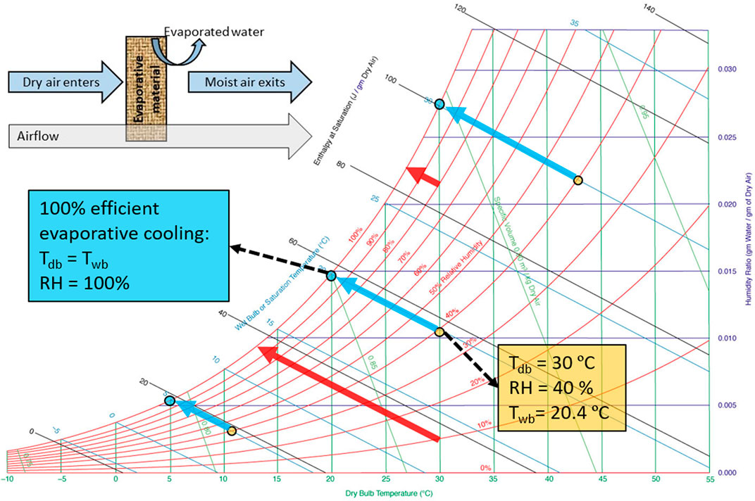
FIGURE 1. Psychrometric chart with an indication of the evaporative cooling process [adapted from (Ogawa, 2021)]. Blue arrows indicate the maximal temperature depression when starting at a relative humidity of 40% for several dry-bulb temperatures. Red arrows indicate the maximal temperature depression at a dry-bulb temperature of 30°C starting at several relative humidities.

Therefore, we present the following design charts for engineers developing evaporative coolers (Figure 2; Figure 3). They present the following parameters as a function of the ambient dry-bulb temperature and relative humidity:

- The wet-bulb temperature (T_wb), so the lowest temperature that can be reached by pure evaporative cooling (Figures 2A, C, E). This value is essential to determine for a certain food to which extent its ideal storage temperature can be reached.

- The temperature depression or drop invoked by evaporative cooling (∆T_ev = T_db-T_wb) (Figures 2B, D, F). This parameter indicates the gain in postharvest life that can be achieved. The Q₁₀ value, namely the ratio between the rate constants of degradation reaction in the food, is typically two to three for fresh foods (Robertson, 2016). This implies that a decrease in temperature by 10 °C from the ambient, through evaporative cooling, typically doubles or triples the postharvest life of fruits and vegetables.

- The resulting gain in postharvest life compared to when the fruit is stored at ambient conditions. This gain is invoked by a specific temperature depression (Figure 3). We calculated this gain according to a kinetic rate law for the following species: apple, banana, mango, and tomato. The details of the quality model are given in the Supplementary Material.

FIGURE 2

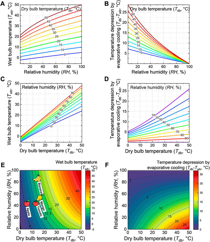
FIGURE 2. Design charts that show parameters as a function of dry-bulb temperature and relative humidity: (A,C,E) wet-bulb temperature, including an indication of optimal storage temperature conditions for several fruits (dotted lines in (e)); (B,D,F) maximal temperature depression invoked by evaporative cooling, namely when the wet-bulb temperature is reached. This image was created using resources from Flaticon.com.

FIGURE 3

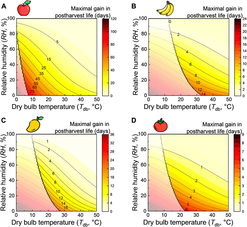
FIGURE 3. The maximal gain in postharvest life when the wet-bulb temperature is reached as a function of dry-bulb temperature and relative humidity for different fruits: (A) apple, (B) banana, (C) mango, and (D) tomato. The stepped black line indicates the optimal storage temperature for the respective fruit. The postharvest life gain is indicated in translucent coloration for the region where the wet-bulb temperature is below the optimal fruit storage temperature since cooling to temperatures lower than the optimal temperature may be detrimental to the fruit due to chilling injury. This image was created using resources from Flaticon.com.

From these results in Figure 2, we can conclude that for a certain humidity, the warmer the region gets, the higher the maximal temperature depression becomes (Figure 2D). This increase is more pronounced in drier areas. The increase in temperature depression with increasing dry-bulb temperature at a constant humidity is almost linear (Figure 2D). The drier the region becomes for a certain dry-bulb temperature, the higher the maximal temperature depression becomes (Figure 2B). The increased temperature depression with decreasing relative humidity is also almost linear (Figure 2B). From Figure 2E, we see that in warm climates (T_db > 25°C), it will be unlikely to reach the ideal storage conditions for several fruits unless the air is very dry. Still, fruit can be stored well below the ambient conditions found under the natural shade. However, the fruit temperature will still be above the recommended conditions. Such storage under lower temperatures will anyway lead to longer shelf life. So even if the ideal temperature is not reached, evaporative cooling provides an advantage. The presented design charts (Figures 2E, F) enable faster identification of the wet-bulb temperature and temperature depression than the traditional psychometric charts since they only depict the wet-bulb temperature. These design charts emulate in fact the different points that otherwise needed to be looked up.

From the results in Figure 3, we see that the temperature reduction induced by evaporative cooling can lead to several days of additional postharvest life. Here the gain in postharvest life implies the additional days gained by storing the fruit in the evaporative cooler at the wet-bulb temperature conditions, as opposed to ambient storage at dry-bulb temperature conditions. The gain in additional postharvest life using passive cooling is remarkable. Even for temperate climates (T_db = 20°C and φ_a = 50%), the postharvest life gain is roughly 2–15 days for the fruits considered. However, this wet-bulb temperature will not be reached in an evaporative cooler due to additional heat sources (e.g., radiation) and non-optimal evaporative cooling. The temperature will also not remain constant throughout the day. Therefore these charts represent the best-case scenario. Nevertheless, adding several days of storage can help farmers sell more of their produce on the markets, leading to less food loss and a higher income for the farmers.

3.2 In which location does it make the most sense to apply evaporative cooling

We tackle a crucial bottleneck in evaporative cooling here: how to scope for regions where evaporative cooling can be successfully applied (Verploegen, 2021b; Verploegen, 2021c). The evaporative cooling potential and its impact on extending the postharvest life of fresh food at a certain location in the world need to be assessed before deploying evaporative cooling. If evaporative cooling is deployed in a region that does not add postharvest life, due to insufficient cooling, farmers will cease to use it and lose trust in the technology. Tools exist to qualitatively assess this cooling potential (Verploegen, 2021b). Our design charts can also identify the temperature depression that can be reached for a certain location worldwide. Using our charts, we can select a specific season or month based on the local environmental conditions (Figure 2; Figure 3). We took the next step forward and calculated and mapped the gain in postharvest life that evaporative cooling gives at every location in India or Nigeria for each month of the year at a resolution of approximately 30 km (section 3.2.1). Furthermore, we developed a similar map for the entire world for four seasons (section 3.2.2). Note that these calculations are based on theoretical estimates, and in the future, a detailed comparison with experimental data is advised.

3.3 Evaporative cooling potential for India and Nigeria

3.3.1 Wet-bulb temperature and maximal temperature depression

Figure 4 indicates the monthly climatic parameters relevant for evaporative cooling under shaded conditions in India and Nigeria, namely the dry-bulb temperature and relative humidity. Figure 5 maps the monthly wet-bulb temperature and the maximal temperature depression achieved by evaporative cooling. We zoom into specific regions in Figure 6.

FIGURE 4

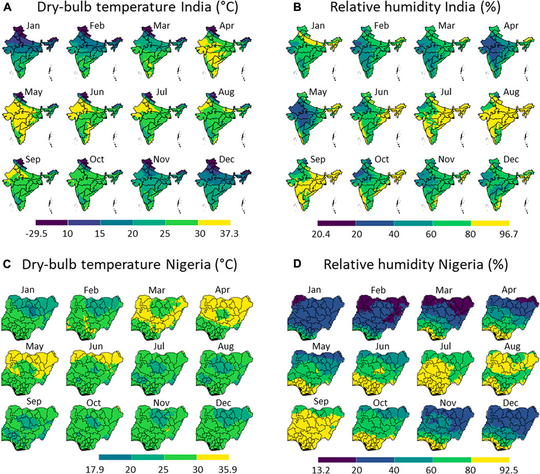
FIGURE 4. Measured data on the local climate, namely the dry-bulb temperature (A,C) and relative humidity (B,D) in India (A,B) and Nigeria (C,D) for each month in 2020. The division of the color scales is based on equal intervals (5 °C for (A,C) and 20% for (B,D)) except for the highest and lowest breaks which are dependent on the max and min values indicated. Created with R Software.

FIGURE 5

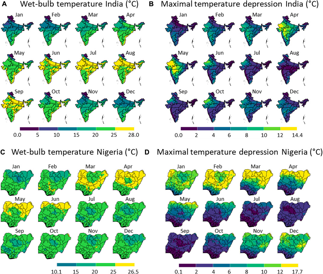
FIGURE 5. Monthly wet-bulb temperature (A,C) and the maximal temperature depression due to evaporative cooling (B,D) in India (A,B) and Nigeria (C,D), showing the example of each month in 2020. The division of the color scales is based on equal intervals (5 °C for (A,C) and 2 °C for (B,D)) except for the highest and lowest breaks which are dependent on the max and min values indicated. Created with R Software.

FIGURE 6

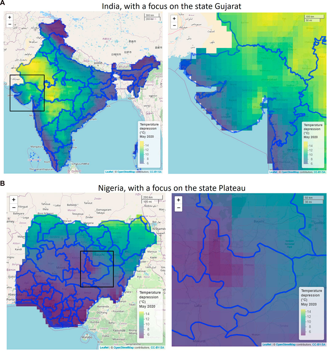
FIGURE 6. Focus of the maximal temperature depression due to evaporative cooling in Gujarat state in India (A) and Plateau state in Nigeria (B) in May 2020. The pixels have a 30-km resolution. Created with R Software.

From these results, we can conclude that with respect to the climate, Nigeria has a few clear dry months (November to April) within almost the entire country. These months will also likely be preferred to apply evaporative cooling. The temperatures are relatively high throughout the year and throughout the country, except for the elevated region in Plateau and Adamawa states. In India, a few drier months are present (February to May), mainly in the country’s northwestern part. The Himalayas cause a very low-temperature zone in the north of the country. As such, both countries have selected months in which evaporative cooling will likely be most efficient.

The maximal temperature depression that can be reached is representative of the gain in postharvest life that we can achieve by evaporative cooling. This depression is the criteria to define the evaporative cooling potential, not the wet-bulb temperature. The temperature depression is strongly correlated with seasonal humidity. We get the highest potential for evaporative cooling in Nigeria between November to April and in India between April and May. In Nigeria, a significant temperature reduction by evaporative cooling can be achieved throughout almost the entire country, except for the coastal region. In India, the largest temperature depression is obtained in the northwestern states (e.g., Gujarat). Here, temperature depressions from ambient, up to 14°C, can be reached due to evaporative cooling. These predictions align with the existing studies on evaporative coolers, where product temperature reductions of typically 3°C–10°C are achieved (see section 1). In many states in India and Nigeria, it is too humid to have a significant temperature reduction (higher than 5°C) by evaporative cooling. This means that if evaporative coolers are applied in these regions, they will have a limited impact on extending the shelf life of fresh produce. As such, farmers might lose trust in deploying this technology. It only makes sense to apply the coolers in regions where a high temperature depression can be achieved. In summary, the highest potential locations to apply evaporative cooling are: (1) for Nigeria, the northern states (Sokoto, Kebbi, Borno, and Yobe) in March and April, and (2) for India, Gujarat, and Madhya Pradesh in April and May. This indicates that each country has its own months and regions in which evaporative cooling will bring the highest gains.

The wet-bulb temperature is also an important parameter, in addition to the maximal temperature depression. It is the lowest storage temperature for fruit and vegetables that can be achieved by evaporative cooling. This produce storage temperature is still relatively high in India and Nigeria in most regions and in months that have the highest potential for evaporative cooling. For India and Nigeria, these temperatures are above about 15°C, so higher than the ideal storage temperatures of most fruits. Therefore, some foods cannot be stored at their optimal temperature with evaporative cooling in these countries. However, a clear reduction of several degrees Celsius can still be obtained when stored in an evaporative cooler at the right location in the country and in the right months. In addition, the higher humidity in the cooler will also help preserve the fruit significantly longer. Typically most fruits should be stored at elevated humidity (80%–95%) to avoid extensive mass loss.

3.3.2 Gain in postharvest life in an evaporative cooler

Figure 7 illustrates the graphical workflow on how the maximal gain in postharvest life in an evaporative cooler is determined. Here we compared to storing fruit at ambient conditions, calculated from the climatic parameters. We illustrated this workflow for banana fruit for a certain month in India. In Figure 8, we show the maximal postharvest life in each month that can be achieved by storing banana fruit in an evaporative cooler in India, so under wet-bulb conditions (similar to Figure 7D). In Figure 9, we show the postharvest life gain (Figure 7E) that can be achieved by storing banana fruit in an evaporative cooler (Figure 7D), compared to at ambient in the shade (Figure 7C). These data indicate where there is the highest potential for reducing the temperature and increasing postharvest life by evaporative cooling in India. We filtered these maps for different states in India with the harvest season for a banana crop (Figure 10). Note that there are regions where evaporative cooling does not add additional postharvest life in these maps since the exterior temperature, when stored in the shade, is already at or below the optimal storage temperature for the fruit of interest. In case the storage temperature in the evaporative cooler fell below the optimal fruit storage temperature, we used this optimal storage temperature for postharvest life calculations.

FIGURE 7

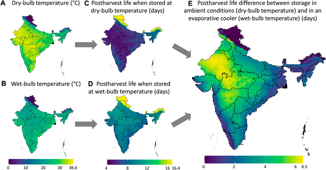
FIGURE 7. The maximal postharvest life in an evaporative cooler calculated from the climatic parameters for banana fruit, showing the example of May 2020. We start from the dry-bulb temperature (A) and wet-bulb temperature (B) to calculate the postharvest life in days (C, D) and then the difference in postharvest life (E). The same color gradients are used for (A, B) and for (C, D). The legends also show the maximum values. Created with R Software.

FIGURE 8

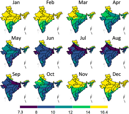
FIGURE 8. Postharvest life in days in an evaporative cooler for each month for banana fruit in India, so when stored at wet-bulb temperature conditions. The division of the color scales is based on equal intervals (2°C) except for the highest and lowest breaks which are dependent on the max and min values indicated. Created with R Software.

FIGURE 9

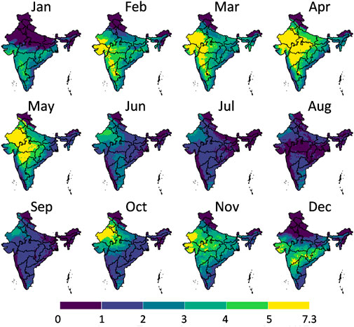
FIGURE 9. The maximal potential gain of the postharvest life in days in each month in India that can be achieved by storing banana fruit in an evaporative cooler compared to ambient temperatures in the shade. The division of the color scales is based on equal intervals (1°C) except for the highest and lowest breaks which are dependent on the max and min values indicated. Created with R Software.

FIGURE 10

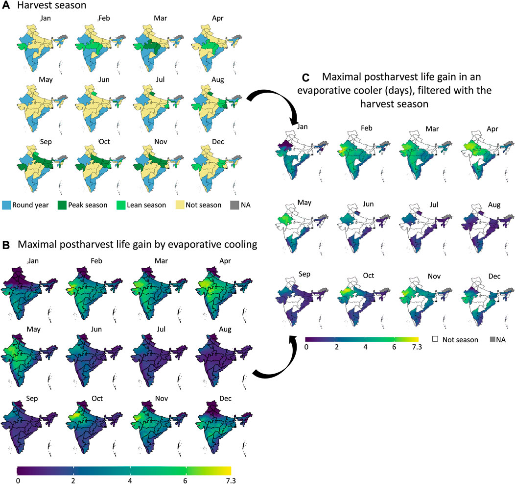
FIGURE 10. Filtering the maximal postharvest life gain by evaporative cooling for banana (B) with the harvest seasons (A) in each state of India. We obtain the maximal postharvest life difference between storage in ambient conditions (dry-bulb temperature) and in an evaporative cooler (wet-bulb temperature) (days) in the states which are in the harvest season (C). The harvest season information (A) was obtained from (Ministery of Commerce and Industry, 2022). Created with R Software.

From the results in these figures, the gain in postharvest life by placing the products in an evaporative cooler is substantial in several regions in the country. Up to 7 days can be gained for bananas, for example. We can thus gain a lot of postharvest life days, so reduce food loss by placing fruit in an evaporative cooler. In a related study (Chopra et al., 2022), the gain in days of storage life was quantified for an entire year for leafy amaranth in India similarly. Filtering our results with the harvesting season proved useful to only target those states where evaporative cooling has a large impact at a certain period of the year. Since the farmers evaluate shelf life on a day-to-day basis, the order of magnitude of days is a sufficient measure (compared to hours or minutes). Note that very perishable fruits, such as berries, are more sensitive to postharvest life predictions, as the time scales for quality decay are different from more resilient species, such as some citrus fruit.

From the results in Figure 11, these regions where the highest evaporative cooling can be achieved for fresh produce also agree to the regions where evaporative cooling is interesting to use for building ventilation in India to improve thermal comfort. This finding stems from a comparison with literature data. A study on 60 cities in India (Hindoliya and Mullick, 2006) quantified in which cities it would make the most sense to use evaporative cooling. The aim was to lower the air temperatures while not increasing the humidity too much to improve the thermal comfort of the people. This study did not consider the efficiency of evaporative cooling but rather identified zones with high ambient temperatures throughout the year and the appropriate relative humidity for evaporative cooling. If we compare our postharvest life gain map with the one for building ventilation potential (Figure 11), we see a lot of parallels.

FIGURE 11

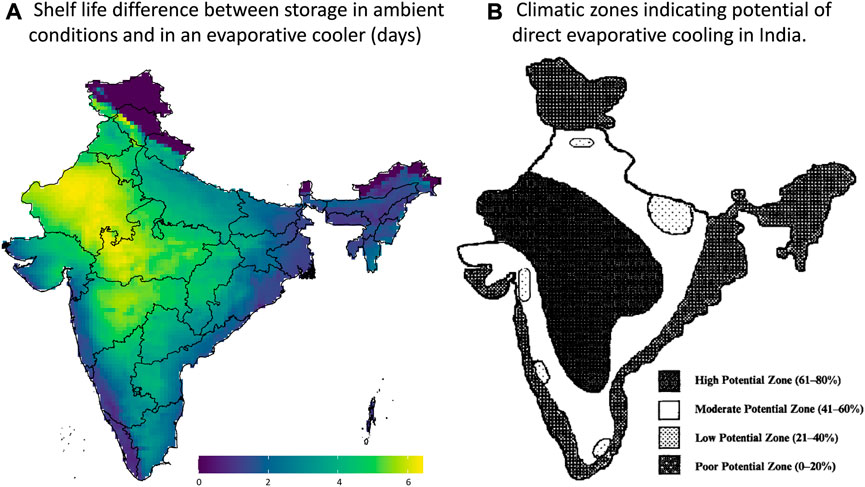
FIGURE 11. (A) Maximal gain in postharvest life by evaporative cooling for banana, showing the example of May 2020. Created with R Software. (B) Climatic zones indicating the potential of direct evaporative cooling in India for the entire year. Reproduced with permission from Hindoliya and Mullick (2006).

3.3.3 Evaporative cooling potential for the world

In addition to India and Nigeria, we also mapped the temperature reduction potential by evaporative cooling for the entire world for May 2020 (Figure 12) as well as for 4 months representing four different seasons (Figure 13). This map clearly shows that the potential and effectiveness of evaporative cooling are strongly dependent on the location and the season in which it is applied. These maps are made openly accessible online (Empa, 2022). More details are found in the Supplementary Material.

FIGURE 12

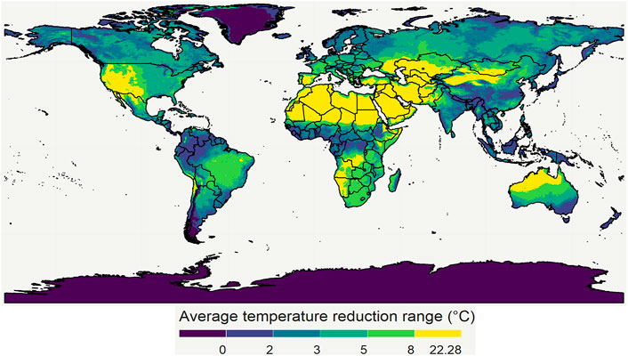
FIGURE 12. The maximal temperature depression due to evaporative cooling for May 2020. The division of the color scales is based on percentiles of all the 2020 monthly average temperature depression data points. 20, 40, 60, and 80 percentiles correspond to 2, 3, 5, and 8°C, respectively. Created with R Software.

FIGURE 13

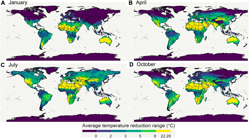
FIGURE 13. The maximal temperature depression due to evaporative cooling for 4 seasons (A–D). The division of the color scales is based on percentiles of all the 2020 monthly average temperature depression data points. 20, 40, 60, and 80 percentiles correspond to 2, 3, 5, and 8°C, respectively. Created with R Software.

From these results, we see that the world has several regions where the temperature can be reduced by more than 8°C. As a result, the shelf life of the produce there can be almost doubled or tripled in these regions, depending on the species and its Q₁₀ value. Note that other researchers have made similar maps to quantify heat exposure and stress of humans, and the impact of loss in working hours, as driven by climate change (Hyatt et al., 2010; Kjellstrom et al., 2018). Here, the computation of their wet-bulb globe temperature and the loss in productivity hours parallels our study’s approach. The aim of making these maps is to give researchers and engineers a first estimate of the possible potential of evaporative cooling, and to sensibilize them for the large differences with the geography.

3.4 How much fruit can 1 L of water cool by evaporation

We aim to quantify how much fruit we can cool with 1 L of water by evaporative cooling. This resulting amount of fruit is depicted in Figure 14 as a function of the dry-bulb temperature and relative humidity for apple fruit. In addition, results for mango, tomato, and banana fruit are also shown on the right-hand side, but the differences were very small.

FIGURE 14

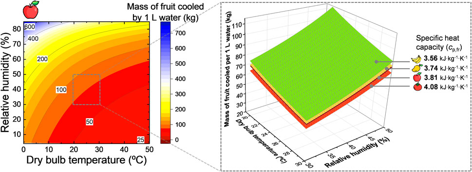
FIGURE 14. Amount of apple fruit [kg] that 1 L of water can cool by evaporative cooling down to the wet-bulb temperature as a function of the environmental conditions where the cooling takes place, namely the dry-bulb temperature and the humidity of the air. The inset on the right shows the effect of the specific heat capacity of fruit for apple, banana, mango, and tomato fruit. This image was created using resources from Flaticon.com.

From these results, we see that 1 L of water can cool down a considerable amount of fruit to the wet-bulb temperature. Note, however, that the wet-bulb temperature might not always be the optimal storage temperature for the fruit. Let us consider a temperature reduction of about 10 °C from the dry-bulb temperature to the wet-bulb temperature. This temperature reduction is achievable by evaporative cooling (Figure 2). Typical conditions in which the wet-bulb temperature drops by 10 °C are, for example, a dry-bulb temperature of about 30 °C and relative humidity of about 40%. When we apply Eq.7, 1 L (or kg) of water can cool down 66 kg of apple fruit by 10 °C. For the same temperature conditions (T_db = 30 °C and φ_a = 40%), we can cool down 71 kg of banana fruit, 68 kg of mango fruit, and 62 kg of tomato fruit by 10 °C ideally. As such, the type of fruit that can be cooled down by 1 L of water does not change so much. Note that these calculations do not consider additional heating by the heat of respiration.

This amount of fruit is the limit to which we can cool as we consider a perfect heat extraction from the fruit with no cooling of the air and no additional heat losses. Even if the cooling potential of this 1 L of water is lower due to these additional losses, the evaporative cooling capacity of water is huge. One liter of water can easily cool down over tenfold of its weight in fruit by 10 °C. Once the fruit is cool, the evaporation of water just needs to maintain the right temperature. The evaporation rate then will strongly depend on various conditions, including the temperature and humidity of the environment.

3.5 What is the cooling power of an evaporative cooler

We aim to quantify the cooling power of an evaporative cooler. We quantify it for a unit cell of a wall of the cooler, so one square meter of wall. We quantify the average cooling power for this unit cell over a specific time. The unit cell is based on our measurements of the charcoal properties and the charcoal cooler we developed previously (Defraeye et al., 2022) but can also be done for other cooling pads. Other cooling pads will then have a different porosity, thickness and moisture content of the pieces of material, which will affect the cooling power. We quantified this average cooling power in Figure 15 as a function of the period over which this water is evaporated (Δt) and the thickness of the walls of a cooler (D_ec).

FIGURE 15

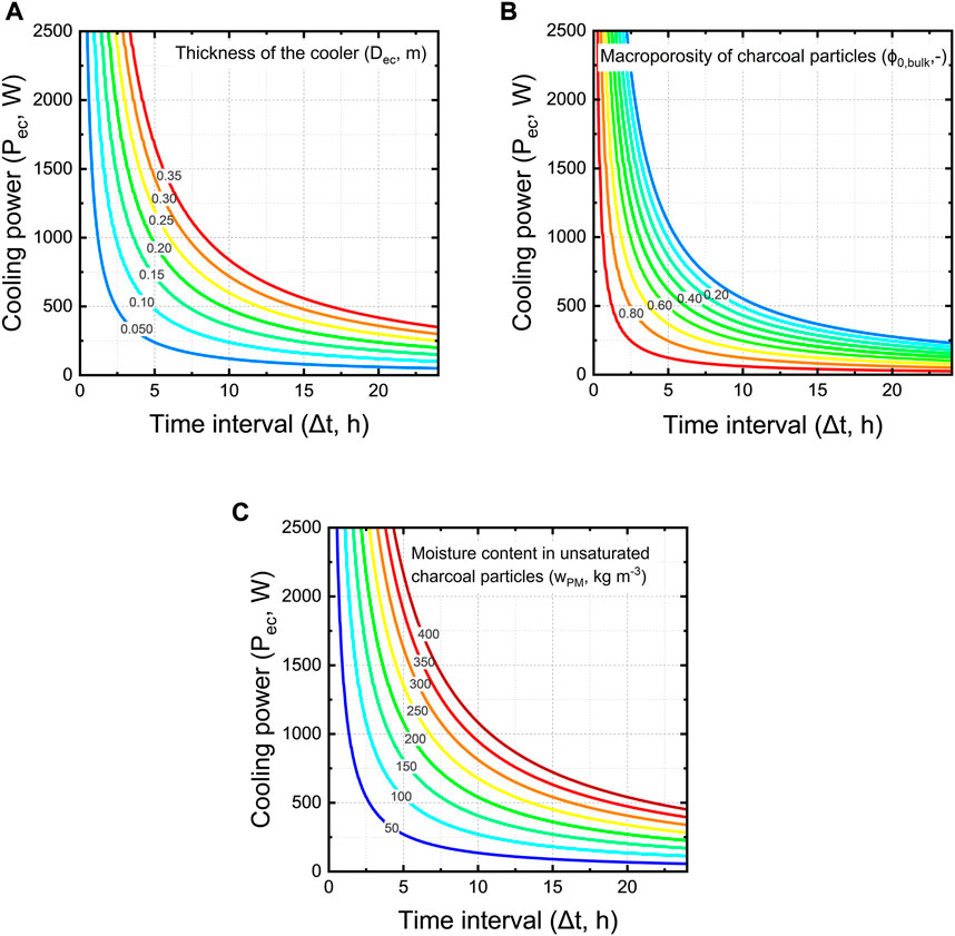
FIGURE 15. Cooling power of a unit cell wall of an evaporative cooler as a function of the period over which this water is evaporated (Δt) for (A) different thickness of the cooler wall (D_ec) at constant bulk porosity of 61% and moisture content of 88 kg m⁻³, (B) different bulk porosity of charcoal pieces (ϕ_0,bulk) at a wall thickness of 10 cm and moisture content of 88 kg m⁻³, and (C) different moisture content of charcoal pieces (w_PM) at a constant bulk porosity of 61% and thickness of 10 cm.

From these results, we see that larger time intervals that would be used for cooling rapidly decrease the cooling power of the evaporative cooler (Figure 15A). A cooler with a thicker wall has a higher cooling capacity for the same time interval. For example, for a time of operation of 5 h, a cooler with a wall thickness of 20 cm has a two times the higher cooling capacity than a cooler with 10 cm walls.

The moisture content of unsaturated charcoal pieces (w_PM) varies strongly depending on the wetting time. We investigated the influence of charcoal moisture content on the cooling power. We varied this parameter between 50 kg m⁻³ and 400 kg m⁻³. Our findings show that the moisture content of charcoal has a large influence on the cooling power, which is logical as more water is available for evaporation (Figure 15C).

A larger macroporosity decreases the cooling capacity of the evaporative cooler (Figure 15B). This is because as the air space between the charcoal pieces (so higher bulk porosity) increases, the bulk moisture content (w_PM,ec) decreases. In turn, there is less water available for evaporation, thus a lower cooling capacity. Increasing the thickness of the cooler wall and reducing the bulk porosity can lead to a higher cooling capacity of the evaporative cooler. When engineers decide which changes in design parameters should be implemented, important factors to consider are the practicability of implementation and the water use efficiency. Thicker cooler walls would require more water to be supplied to the cooler.

In summary, we can reach a cooling power of several hundred Watts with one square meter of cooler, which is substantial. We only quantified the average cooling capacity over a specific time interval. We can not, however, guarantee that this cooling capacity can be reached as this implies the amount of water can be evaporated in that amount of time. We cannot control the time interval over which the cooling occurs, as this depends on the environmental conditions and the airspeed, among others. Our time frames assume the conditions are such that this amount can be evaporated. Note also that this cooling power is not directly transmitted to the product to be cooled. Finally, note that the heat of respiration produced by the fruit can introduce additional heat to be removed. For example, the heat of respiration for bananas is about 55 W tonne⁻¹ at 13°C and 119 W tonne⁻¹ at 20 °C (Kader, 1996). Compared to the cooling power of a cooling blanket of several square meters, these amounts are rather small.

3.6 How does the airflow rate through an evaporative cooler affect its optimal wall thickness

We plot a design chart for calculating the optimal thickness of the walls of the evaporative cooler, given a certain bulk porosity and airspeed (Figure 16). An optimal wall thickness implies that, under the local airflow conditions at that specific location, the maximal cooling efficiency is reached. The airspeed through the cooler is defined by the local airflow conditions. We assume one square meter of a wall of the evaporative cooler (A_ec = 1 m²) and a spherical charcoal piece size (D_cc) of 80 mm. We consider airspeeds ranging between 0.01 and 5 m s⁻¹.

FIGURE 16

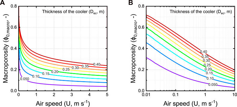
FIGURE 16. The optimal wall thickness of the evaporative cooler as a function of the approach flow airspeed (U, m s⁻¹) and bulk porosity (ϕ_0,bulk, -), for charcoal pieces of 80 mm on a (A) linear and (B) logarithmic scale.

From these results, we see that in regions where airspeeds are low and are typically varying during the day around these low values, optimal performance will be difficult to achieve. The reason is that with a slight change of airspeed, the optimal wall thickness largely varies. As an example, for an evaporative cooler with a bulk porosity of 40% operating in a region with an airspeed of 0.1 m s⁻¹, the optimal blanket thickness would be 76 mm. The optimal blanket thickness would be 350 mm for an evaporative cooler with a bulk porosity of 40% operating in a region with an airspeed of 0.5 m s⁻¹. Once built, we can not change the wall thickness or bulk porosity. That way, the performance will just vary strongly with airspeed. However, we find that the optimal wall thickness becomes much more independent of the bulk porosity at higher airspeeds. For example, a 50 mm thick cooler requires about the same bulk porosity for airspeeds above 1 m s⁻¹.

Note that the optimal wall thickness is independent of T_db and φ_a. This implies that the environmental conditions will not determine the required optimal wall thickness. As such, a cooler with an optimized wall thickness for specific airflow conditions will perform similarly in different climates. We can, thereby, design a cooler based on local wind conditions and deploy it in regions with similar airflow conditions around the world.

Such design charts are useful to evaluate for a certain region (country, urban, rural) or location (free field, building roof) with a certain airspeed how thick the walls of an evaporative (charcoal) cooler should be. This optimal wall thickness implies optimal efficiency, so the lowest possible temperature and a high cooling capacity. Note that our quantification of the optimal wall thickness was based on analytical equations. Future steps should be to verify this experimentally or with physics-based simulations. The reason is that the complex transient heat and mass balances cannot be captured fully with simplified analytical equations.

4 Conclusion

Passive evaporative cooling has a huge potential for helping to preserve fresh fruit and vegetables longer after harvest. Single households, smallholder farmers, and farmer cooperatives in developing countries or remote areas can benefit especially. For direct evaporative coolers, the extended postharvest life only becomes apparent in specific conditions. The evaporative cooler should be used in a location with the right environmental conditions and at the right time of the year to enable sufficient cooling. Our design charts of the temperature depression answer how much evaporative cooling can maximally drop the temperature and extend postharvest life for a certain crop. We mapped this for India, Nigeria, and the entire world, by which we quickly can target the best locations and months for evaporative cooling. Such easy-to-use tools are essential during scoping regions for evaporative cooling to avoid disillusions with service providers, policymakers, farmer groups, or cooperatives. Installing evaporative coolers in regions and periods of the year with low potential and disappointing performance are potential causes for farmers' limited adoption of this technology. With the information we presented in this work, stakeholders can answer the two most important questions quickly when scoping for evaporative cooling sites: (1) how much can we maximally decrease the fruit storage temperature compared to storing outside under the natural shade, so how much postharvest life can we actually gain here; (2) what is the lowest storage temperature at a specific site and period of the year, and how far is this from the ideal storage temperature of that crop.

Once a suitable region is identified, our other design charts enable us to optimally determine the wall thickness of the evaporative cooler based on the local airspeed to have the optimal evaporation rate. Here there is a trade-off between increasing efficiency, so lowering the temperature, and increasing cooling power. However, the target for fresh fruit and vegetables is to maximize temperature drop and humidity levels, not maximizing the cooling capacity. Note that the calculations in the present study were based on theoretical estimates. Despite the fact that our predictions align with the values of other studies, verification and comparison with experiments is advised in the future. Another future aim should be to identify how the farmer adoption of the evaporative cooling technology is linked to the resulting temperature depression that is achieved. Do farmers adopt the solution if they can decrease the temperature by 5 °C below ambient? Or should this be by 10 °C below ambient or even more?

The information presented in this study aims to catalyze the development of small-scale evaporative coolers. Only then can we make passive postharvest cooling accessible to the currently-underserved rural, peri-urban and urban marginal and smallholder farmers. These stakeholders need to see that evaporative coolers bring significant gains in postharvest life, reduce food losses, and increase revenues. They also need to see that evaporative coolers do not perform well in certain locations in their country and at certain months of the year. We need to install the coolers only in regions where they help save food and operate them in the most optimal months. Such evidence-based success stories are essential to building trust in this technology. Apart from the farmers, governments and organizations that disseminate passive cooling technologies, among others, need to be convinced of their potential to communicate to farmers convincingly.

Author’s Note

This manuscript has been released as a preprint on engrXiv.

Data availability statement

The raw data supporting the conclusions of this article will be made available by the authors, without undue reservation.

Author contributions

TD conceptualized the study and acquired funding; TD did the project administration; TD, CS, and KS performed the investigation, developed the methodology, and executed the modeling; TD wrote the original draft of the paper, with key input from CS and KS; KS and CS did the visualization; SS, DO performed critical review and editing. All authors contributed to the article and approved the submitted version.

Funding

This work was funded partially by the data.org Inclusive Growth and Recovery Challenge grant "Your Virtual Cold Chain Assistant". Open access funding provided by Empa - Swiss Federal Laboratories for Materials Science and Technology. This work was supported by The Rockefeller Foundation and the Mastercard Center for Inclusive Growth, as well as by the project “Scaling up Your Virtual Cold Chain Assistant” commissioned by the German Federal Ministry for Economic Cooperation and Development and being implemented by BASE and Empa on behalf of the German Agency for International Cooperation (GIZ). The funders were not involved in the study design, collection, analysis, interpretation of data, the writing of this article, or the decision to submit it for public.

Conflict of interest

The authors declare that the research was conducted in the absence of any commercial or financial relationships that could be construed as a potential conflict of interest.

Publisher’s note

All claims expressed in this article are solely those of the authors and do not necessarily represent those of their affiliated organizations, or those of the publisher, the editors and the reviewers. Any product that may be evaluated in this article, or claim that may be made by its manufacturer, is not guaranteed or endorsed by the publisher.

Supplementary material

The Supplementary Material for this article can be found online at: https://www.frontiersin.org/articles/10.3389/frfst.2023.1100181/full#supplementary-material

References

Abaranji, S., Panchabikesan, K., and Ramalingam, V. (2021). Experimental study on the direct evaporative air-cooling system with vermicompost material as the water storage medium. Sustain. Cities Soc. 71, 102991. doi:10.1016/j.scs.2021.102991

CrossRef Full Text | Google Scholar

Adekanye, T., Babaremu, K., and Okunola, A. (2019). Evaluation of an active evaporative cooling device for storage of fruits and vegetables. Agric. Eng. Int. CIGR J. 21, 203–208.

Google Scholar

Alam, M. F., Sazidy, A. S., Kabir, A., Mridha, G., Litu, N. A., and Rahman, M. A. (2017). An experimental study on the design, performance and suitability of evaporative cooling system using different indigenous materials. AIP Conf. Proc. 1851. doi:10.1063/1.4984704

CrossRef Full Text | Google Scholar

Allen, R. G., Walter, I. A., Elliott, R. L., Howell, T. A., Itenfisu, D., Jensen, M. E., et al. (2005). The ASCE standardized reference evapotranspiration equation. ASCE Stand. Ref. Evapotranspiration Equ., 1–203. doi:10.1061/9780784408056

CrossRef Full Text | Google Scholar

Allen, R., Pereira, L., Raes, D., and Smith, M. (1998). Crop evapotranspiration - guidelines for computing crop water requirements - FAO Irrigation and drainage paper 56, Evapotranspiración del cultivo Guías para la determinación de los requerimientos de agua de los cultivos, 56. Rome: ESTUDIO FAO RIEGO Y DRENAJE.

Google Scholar

Ambuko, J., Wanjiru, F., Chemining’wa, G. N., Owino, W. O., and Mwachoni, E., 2017. Preservation of postharvest quality of leafy amaranth (Amaranthus spp.) vegetables using evaporative cooling. J. Food Qual. 2017, 1–6. doi:10.1155/2017/5303156

CrossRef Full Text | Google Scholar

Anyanwu, E. E. (2004). Design and measured performance of a porous evaporative cooler for preservation of fruits and vegetables. Energy Convers. Manag. 45, 2187–2195. doi:10.1016/j.enconman.2003.10.020

CrossRef Full Text | Google Scholar

Boettiger, S., and Sanghvi, S. (2019). How digital innovation is transforming Indian agriculture. McKinsey, McKinsey & Company report.

Google Scholar

Chinenye, N. M. (2011). Development of clay evaporative cooler for fruits and vegetables preservation. Agric. Eng. Int. CIGR J. 13, 1–8.

Google Scholar

Chinenye, N. M., Manuwa, S. I., Olukunle, O. J., and Oluwalana, I. B. (2013). Development of an active evaporative cooling system for short-term storage of fruits and vegetable in a tropical climate. Agric. Eng. Int. CIGR J. 15, 307–313.

Google Scholar

Chopra, S., Müller, N., Dhingra, D., Mani, I., Kaushik, T., Kumar, A., et al. (2022). A mathematical description of evaporative cooling potential for perishables storage in India. Postharvest Biol. Technol. 183, 111727. doi:10.1016/j.postharvbio.2021.111727

CrossRef Full Text | Google Scholar

Dadhich, S. M., Dadhich, H., and Verma, R. C. (2008). Comparative study on storage of fruits and vegetables in evaporative cool chamber and in ambient. Int. J. Food Eng. 4, 1–22. doi:10.2202/1556-3758.1147

CrossRef Full Text | Google Scholar

Defraeye, T., Schudel, S., Shrivastava, C., Motmans, T., Umani, K., Crenna, E., et al. (2022). The charcoal cooling blanket: A scalable, simple, self-supporting evaporative cooling device for preserving fresh foods. engrXiv. Available at: https://engrxiv.org/preprint/view/2221.

Google Scholar

Deoraj, S., Ekwue, E. I., and Birch, R. (2015). An evaporative cooler for the storage of fresh fruits and vegetables. West Indian J. Eng. 38, 86.

Google Scholar

Elansari, A. M., Yahia, E. M., and Siddiqui, W. (2019). “Chapter 12 - storage systems,” in Postharvest technology of perishable horticultural commodities (Woodhead Publishing), 401–437. doi:10.1016/B978-0-12-813276-0.00012-2

CrossRef Full Text | Google Scholar

Empa (2022). Evaporatieve cooling potential map [WWW Document]. URL. Available at: https://empasimbiosys.github.io/evapo_cooling_map/.

Google Scholar

Getinet, H., Seyoum, T., and Woldetsadik, K. (2008). The effect of cultivar, maturity stage and storage environment on quality of tomatoes. J. Food Eng. 87, 467–478. doi:10.1016/j.jfoodeng.2007.12.031

CrossRef Full Text | Google Scholar

GKI (2017). Innovating the future of food systems - a global scan for the innovations needed to transform food systems in emerging markets by 2035.

Google Scholar

Goedde, L., Ooko-Ombaka, A., and Pais, G. (2019). Winning in africa’s agricultural market. McKinsey & Company report.

Google Scholar

Hindoliya, D. A., and Mullick, S. C. (2006). Assessment of utilisation potential of direct evaporative cooling for India. Int. J. Ambient. Energy 27, 21–28. doi:10.1080/01430750.2006.9674998

CrossRef Full Text | Google Scholar

Hyatt, O. M., Lemke, B., and Kjellstrom, T. (2010). Regional maps of occupational heat exposure: Past, present, and potential future. Glob. Health Action 3, 5715. doi:10.3402/gha.v3i0.5715

PubMed Abstract | CrossRef Full Text | Google Scholar

Jain, D. (2007). Development and testing of two-stage evaporative cooler. Build. Environ. 42, 2549–2554. doi:10.1016/j.buildenv.2006.07.034

CrossRef Full Text | Google Scholar

Jensen, M. E., Burman, R. D., and Allen, R. G. (1990). Evapotranspiration and irrigation water requirements. New York.

Google Scholar

Kader, A. A. (1996). Fruit produce facts - UC postharvest technology center [WWW document].

Google Scholar

Kanali, C., Kituu, G., Mutwiwa, U., Mung’atu, J., Ronoh, E., Njuguna, S., et al. (2017). RE4Food project: Energy efficient rural food processing utilising renewable energy to improve rural livelihoods in Kenya.

Google Scholar

Kjellstrom, T., Freyberg, C., Lemke, B., Otto, M., and Briggs, D. (2018). Estimating population heat exposure and impacts on working people in conjunction with climate change. Int. J. Biometeorol. 62, 291–306. doi:10.1007/s00484-017-1407-0

PubMed Abstract | CrossRef Full Text | Google Scholar

Korir, M. K., Mutwiwa, U. N., Kituu, G. M., and Sila, D. N. (2017). Effect of near infrared reflection and evaporative cooling on quality of mangoes. Agric. Eng. Int. CIGR J. 19, 162–168.

Google Scholar

Manuwa, S. I., and Odey, S. O. (2012). Evaluation of pads and geometrical shapes for constructing evaporative cooling system. Mod. Appl. Sci. 6, 45–53. doi:10.5539/mas.v6n6p45

CrossRef Full Text | Google Scholar

Ministery of Commerce and Industry (2022). Harvesting season of banana [WWW Document]. URL. Available at: https://apeda.gov.in/apedawebsite/six_head_product/Harvesting_Season_Banana.htm.

Google Scholar

Mittal, A., Kataria, T., Das, G. K., and Chatterjee, S. G. (2006). Evaporative cooling of water in a small vessel under varying ambient humidity. Int. J. Green Energy 3, 347–368. doi:10.1080/01971520600704654

CrossRef Full Text | Google Scholar

Mogaji, T. S., and Fapetu, O. P. (2011). Development of an evaporative cooling system for the preservation of fresh vegetables. Afr. J. Food Sci. 5, 255–266.

Google Scholar

Mogaji, T. S., Olufemi, A. D., and Fapetu, O. P. (2013). Marketing performance and efficiency of evaporative-preservation cooling system for fresh tomato marketing in Ondo State, Nigeria. Afr. J. Agric. Res. 8, 468–474. doi:10.5897/AJAR12.1308

CrossRef Full Text | Google Scholar

Mujuka, E., Ambuko, P. J., Mburu, P. J., and Ogutu, P. A. (2021). Investment in technologies: Key strategy for. Postharvest Loss Reduct. 2, 47–48.

Google Scholar

Nkolisa, N., Magwaza, L. S., Workneh, T. S., and Chimpango, A. (2018). Evaluating evaporative cooling system as an energy-free and cost-effective method for postharvest storage of tomatoes (Solanum lycopersicum L.) for smallholder farmers. Sci. Hortic. Amst. 241, 131–143. doi:10.1016/j.scienta.2018.06.079

CrossRef Full Text | Google Scholar

Ogawa, A. (2021). Psychrometric chart at sea level in SI units [WWW Document]. URL. Available at: https://commons.wikimedia.org/wiki/File:PsychrometricChart-SeaLevel-SI.jpg.

Google Scholar

Ogbuagu, N., Green, I., Anyanwu, C., and Ume, J. (2016). Performance evaluation of a composite-padded evaporative cooling storage bin. Niger. J. Technol. 36, 302–307. doi:10.4314/njt.v36i1.37

CrossRef Full Text | Google Scholar

Olosunde, W. A., Aremu, A. K., and Onwude, D. I. (2016). Development of a solar powered evaporative cooling storage system for tropical fruits and vegetables. J. Food Process. Preserv. 40, 279–290. doi:10.1111/jfpp.12605

CrossRef Full Text | Google Scholar

Olosunde, W. A., Igbeka, J. C., and Olurin, T. O. (2009). Performance evaluation of absorbent materials in evaporative cooling system for the storage of fruits and vegetables. Int. J. Food Eng. 5. doi:10.2202/1556-3758.1376

CrossRef Full Text | Google Scholar

Patel, N., Mindhe, O., Lonkar, M., Naikare, D., Pawar, S., Bhojwani, V. K., et al. (2021). “Performance investigation of mitticool refrigerator,” in Techno-societal 2020 (Springer), 1051–1061.

CrossRef Full Text | Google Scholar

Poku, R., Oyinki, W., and Ogbonnaya, T., A. E. (2017). The effects of evaporative cooling in tropical climate. Am. J. Mech. Eng. 5, 145–150. doi:10.12691/ajme-5-4-5

CrossRef Full Text | Google Scholar

Raza, H. M. U., Sultan, M., Bahrami, M., and Khan, A. A. (2021). Experimental investigation of evaporative cooling systems for agricultural storage and livestock air-conditioning in Pakistan. Build. Simul. 14, 617–631. doi:10.1007/s12273-020-0678-2

CrossRef Full Text | Google Scholar

Rehman, D., McGarrigle, E., Glicksman, L., and Verploegen, E. (2020). A heat and mass transport model of clay pot evaporative coolers for vegetable storage. Int. J. Heat. Mass Transf. 162, 120270. doi:10.1016/j.ijheatmasstransfer.2020.120270

CrossRef Full Text | Google Scholar

Ricciardi, V., Ramankutty, N., Mehrabi, Z., Jarvis, L., and Chookolingo, B. (2018). How much of the world’s food do smallholders produce? Glob. Food Sec 17, 64–72. doi:10.1016/j.gfs.2018.05.002

CrossRef Full Text | Google Scholar

Robertson, G. L. (2016). Food packaging: Principles and practice Third Edit. ed. Boca-Raton: Taylor & Francis Group LLC. doi:10.1177/0340035206070163

CrossRef Full Text | Google Scholar

Sadeghi, S. H., Peters, T. R., Cobos, D. R., Loescher, H. W., and Campbell, C. S. (2013). Direct calculation of thermodynamic wet-bulb temperature as a function of pressure and elevation. J. Atmos. Ocean. Technol. 30, 1757–1765. doi:10.1175/JTECH-D-12-00191.1

CrossRef Full Text | Google Scholar

Samira, A., Woldetsadik, K., and Workneh, T. S. (2013). Postharvest quality and shelf life of some hot pepper varieties. J. Food Sci. Technol. 50, 842–855. doi:10.1007/s13197-011-0405-1

PubMed Abstract | CrossRef Full Text | Google Scholar

Shitanda, D., Oluoch, O. K., and Pascall, A. M. (2011). Performance evaluation of a medium size charcoal cooler installed in the field for temporary storage of horticultural produce. Agric. Eng. Int. CIGR J. 13, 1–8.

Google Scholar

Sibanda, S., and Seyoum Workneh, T. (2021). The influence of indirect air-cooling combined with evaporative cooling on tomato fruit cooling time and temperature. J. Agric. Crop. 7, 69–75. doi:10.32861/jac.72.69.75

CrossRef Full Text | Google Scholar

Sibanda, S., and Workneh, T. S. (2019). Effects of indirect air cooling combined with direct evaporative cooling on the quality of stored tomato fruit. CYTA - J. Food 17, 603–612. doi:10.1080/19476337.2019.1622595

CrossRef Full Text | Google Scholar

Simões-Moreira, J. R. (1999). A thermodynamic formulation of the psychrometer constant. Meas. Sci. Technol. 10, 302–311. doi:10.1088/0957-0233/10/4/008

CrossRef Full Text | Google Scholar

Stull, R. (2011). Wet-bulb temperature from relative humidity and air temperature. J. Appl. Meteorol. Climatol. 50, 2267–2269. doi:10.1175/JAMC-D-11-0143.1

CrossRef Full Text | Google Scholar

Teutsch, B., and Kitinoja, L. (2019). 100 under 100$ - tools for reducing postharvest losses. The Postharvest Education Foundation.

Google Scholar

Vanndy, M., Buntong, B., Chanthasombath, T., Sanatem, K., Acedo, A., and Weinberger, K. (2008). Evaporative cooling storage of tomato in Cambodia and Laos. Acta Hortic., 565–570. doi:10.17660/actahortic.2008.804.83

CrossRef Full Text | Google Scholar

Verploegen, E. (2021a). Affordable, scalable, overlooked: Evaporative cooling can fight food loss – why isn’t the development sector embracing it? [WWW document]. URL. Available at: https://d-lab.mit.edu/news-blog/blog/affordable-scalable-overlooked-evaporative-cooling-can-fight-food-loss-why-isnt.

Google Scholar

Verploegen, E. (2021c). Determining if evaporative cooling has the potential to provide value in a specific context [WWW Document]. URL. Available at: https://d-lab.mit.edu/research/food/evaporative-cooling-vegetable-preservation/suitability-scoping.

Google Scholar

Verploegen, E. (2021b). Evaporative cooling for vegetable preservation [WWW document]. URL. Available at: https://d-lab.mit.edu/research/evaporative-cooling-vegetable-preservation.

Google Scholar

Zakari, M. D., Abubakar, Y. S., Muhammad, Y. B., Shanono, N. J., Nasidi, N. M., Abubakar, M. S., et al. (2016). Design and construction of an evaporative cooling system for the storage of fresh tomato. ARPN J. Eng. Appl. Sci. 11, 2340–2348.

Google Scholar