 Asif Mushtaq
 Amna Noreen
 Kåre Olaussen
- 1Seksjon for Matematikk, Nord Universitet, Bodø, Norway
- 2Bodin videregående skole, Nordland fylkeskommune, Bodø, Norway
- 3MJAU, Trondheim, Norway
A large class of problems in quantum physics involve solution of the time independent Schrödinger equation in one or more space dimensions. These are boundary value problems, which in many cases only have solutions for specific (quantized) values of the total energy. In this article we describe a Python package that “automagically” transforms an analytically formulated Quantum Mechanical eigenvalue problem to a numerical form which can be handled by existing (or novel) numerical solvers. We illustrate some uses of this package. The problem is specified in terms of a small set of parameters and selectors (all provided with default values) that are easy to modify, and should be straightforward to interpret. From this the numerical details required by the solver is generated by the package, and the selected numerical solver is executed. In all cases the spatial continuum is replaced by a finite rectangular lattice. We compare common stensil discretizations of the Laplace operator with formulations involving Fast Fourier (and related trigonometric) Transforms. The numerical solutions are based on the NumPy and SciPy packages for Python 3, in particular routines from the scipy.linalg, scipy.sparse.linalg, and scipy.fftpack libraries. These, like most Python resources, are freely available for Linux, MacOS, and MSWindows. We demonstrate that some interesting problems, like the lowest eigenvalues of anharmonic oscillators, can be solved quite accurately in up to three space dimensions on a modern laptop—with some patience in the 3-dimensional case. We demonstrate that a reduction in the lattice distance, for a fixed the spatial volume, does not necessarily lead to more accurate results: A smaller lattice length increases the spectral width of the lattice Laplace operator, which in turn leads to an enhanced amplification of the numerical noise generated by round-off errors.
1. Introduction
The Schrödinger equation has been a central part of “modern” physics for almost a century. When interpreted broadly, it can be formulated in a multitude of ways [1]. Here we mainly restrict our discussion to the non-relativistic, time independent form,
This constitutes an eigenvalue problem for E (there are many cases where the operator defined by Equation (1) allows for a continuous spectrum of E-values, but this will not directly influence the treatment of finite discretizations of such systems). In Equation (1), q denotes the configuration space coordinate for a system of one or more particles in one or more spatial dimensions, and Δq is a Laplace operator on this configuration space. V(q) is the interaction potential, and E the eigenvalue parameter, interpreted as an allowed energy for the quantum system.
Despite its appearance as a single-particle equation, Equation (1) can also be used to model N-particle systems, with q = (r1, …, rN) and Δq = (c1Δ1, …, cNΔN). Here each Δk is an ordinary flat space Laplace operator, and ck is a numerical coefficient inversely proportional to the mass mk of particle k; this mass may differ from particle to particle. By a suitable scaling of each coordinate rk, one can mathematically transform all ck to (for instance) unity. But such transformations may obscure physical interpretations of the coordinates, and make mathematical formulations more error-prone.
How to solve eigenvalue problems like (1)? Fortunately for the rapid initial development of quantum mechanics, for many important physical cases [like the hydrogen atom [2, 3] and harmonic oscillators [4]] it could be reduced to a set of one-dimensional eigenvalue problems, through the separation of variables method. Moreover, the resulting one-dimensional problems could all be solved exactly by analytic methods. The origins for such fortunate states of affairs can invariably be traced to an enhanced set of symmetries. However, not every system of physical interest enjoy a high degree of symmetry. Even most one-dimensional problems of the form (1) have no known analytic solution. A popular and much investigated system is the anharmonic oscillator,
This model has often functioned as a theoretical laboratory [5, 6], for instance to investigate the behavior and properties of perturbative [7, 8] and other [9–12] expansions, and alternative solution methods [13–15].
It this article we describe some attempts to simplify numerical solutions of eigenvalue problems like (1). Our approach relies on standard numerical algorithms, already coded and freely available through Python packages like numpy [16] and scipy [17, 18]. The main aim is to automatize the transformation of (1) to function calls accepted by the numerical eigenvalue solvers. Within the above class of models, the problem is completely defined by the coefficient vector (c1, c2, …, cN) and the real function V(q). In principle, this should be the only user input required for a numerical solution.
In practice some additional decisions must be made, like how a possibly infinite configuration space should be reduced to a region of finite extent, how the boundaries of this region should be treated, and how this region should be further approximated by a finite lattice. Other options involve selection of numerical approaches, like whether dense or iterative sparse matrix solvers should be used. Such decisions have consequences for many “trivial” details of the numerical programs, but they can be provided in the form of parameters and selectors, automatically implemented without further tedious and error-prone human intervention. Even many of the decisions indicated above may ultimately by delegated to artificial intelligence systems, but this is beyond our current scope.
2. Available Python Procedures for Numerical Solution
Numerical approaches to problems like those above are in principle straightforward: The operator
defined by Equation (1) is approximated by a finite real symmetric matrix
where we have introduced the symbol T = −Δq. For densely defined matrices MH there are several standard numerical eigenvalue solvers available, like eig and eigvals in the scipy.linalg package. A 104 × 104 matrix of double precision numbers requires 800 Mb of storage space; this is indicative of the problem magnitudes that can be handled by dense matrix methods on (for instance) modern laptops. That is, such computers have more than enough memory for numerical treatment of one-dimensional problems, and usually also sufficient memory for two-dimensional ones.
For higher-dimensional problems one may utilize the sparse nature of MH to find solutions through iterative procedures, like the eigsh eigenvalue solver in the scipy.sparse.linalg package. This solver does not require any explicit matrix construction of MH, only a LinearOperator function that returns the vector MHψ for any input vector ψ. In the representations we consider, MV is always diagonal, and MT can be made diagonal by a Fast Fourier Transform (FFT), or some of its discrete trigonometric variants. This opens the possibility it to handle non-sparse matrix problems, where T is replaced by more general expressions of F(T), by the same procedures. For instance functions F that involves fractional and/or inverse powers of its arguments.
3. Required Parameters and Selectors
In this section we describe the additional quantities that a user must input for a full specification of the numerical problem. They assume that configuration space has been modeled by a rectangular point lattice, with a selection of possible boundary conditions.
3.1. Lattice Shape
The most basic quantity of the numerical model is the discrete lattice approximating the relevant region of configuration space. For rectangular approximations this is defined by the shape parameter, a Python tuple,
where each sk is a positive integer specifying the number of lattice points in the k'th direction, and d is the (effective) dimension of configuration space. For models with continuous symmetries (for instance rotational ones) the effective dimension may be chosen smaller than the physical one, by separation of variables. Likewise, discrete symmetries may can used to reduce the size of configuration space that this lattice must approximate.
In Python programs, quantities like the wave function ψ and the potential V are defined as floating point NumPy arrays of shape shape.
3.2. Edge Lengths and Offsets
The geometric extent of the selected region is specified by its edge lengths xe. This is a NumPy array of positive floating point numbers,
A secondary quantity, derived from xe and shape is the elementary lattice cell,
The absolute positioning of the region, with respect to some fixed coordinate system, is specified by a NumPy array of floating point numbers,
This is defined as the position of the “lower left” corner of the selected region. The placement of the lattice points within the region still needs to be specified, as will be discussed below.
3.3. Boundary Conditions
The restriction to finite regions of space requires imposition of boundary conditions. For regions of rectangular shape (generalized to arbitrary dimensions), as considered here, the perhaps simplest choice is periodic boundary conditions in each directions. This may be viewed as a topological property of configuration space itself. Other boundary conditions are really properties of functions defined on this space, as specifications of how the functions should be extended beyond the boundary. Two natural choices are symmetric and anti-symmetric extensions. With a lattice approximation a further distinction can be made, related to how the lattice points are positioned relative to the boundary.
In this connection, it is natural to consider the cases handled by the trigonometric cousins of the fast Fourier transform (FFT). In the one-dimensional case the extension may be symmetric or anti-symmetric with respect to a boundary, which is situated either (i) at a lattice point, or (ii) midway between two lattice points. Thus, at each boundary there is 2 × 2 matrix of possibilities, as indicated by Table 1.
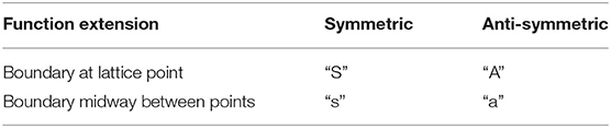
Table 1. Individual boundary conditions covered by standard discrete trigonometric transforms (DCT and DST).
With two boundaries there are altogether 4 × 4 = 16 possibilities. However, the routines in scipy.fftpack (dct and dst of types I–IV) only implement cases where both options come from the same row of Table 1. With the periodic extension P in addition, one ends up with a set of nine possibilities in each direction:
Hence, the numerical model must be further specified by a Python tuple of two-character strings, defining the selected boundary condition in all directions,
with each (or in an enlarged set of possibilities).
3.4. Lattice Positions. Dual Lattice Squared Positions
When bc is given, one may automatically calculate the positions of all lattice points
provided shape, xe, and xo are also known. In Equation (9), the property xlat is a tuple of one-dimensional arrays. For illustration, consider the case of a 3-dimensional lattice of shape (sx, sy, sz). Then xlat is a Python tuple (X, Y, Z), where X is a numpy array of shape (sx, 1, 1), Y is a numpy array of shape (1, sy, 1), and Z is a numpy array of shape (1, 1, sz). These are all one-dimensional arrays, but their shape information implies that (for instance) the Python expression X*Y automatically evaluates to a numpy array of shape (sx, sy, 1).
A Python function V(x, y, z), defined by an expression that can involve “standard” functions, may then be evaluated on the complete lattice by the short and simple expression V(*xlat). When V depends on all its arguments, the result will be a numpy array of shape (sx, sy, sz).
In general, when Fourier transforming a periodic function f(x), where x takes values on some discrete lattice, the result becomes another periodic function , where k takes values on another discrete lattice (the dual lattice/reciprocal space). Modulo an overall scaling, a set of k-values (labeling the points of some complete, minimal subdomain to be extended by periodicity) can be defined such that f(x + a) transforms to . A natural choice for that minimal domain is, in physicists language, the first Brillouin zone (this choice may still leave a somewhat arbitrary selection of boundary points to be included). On this subdomain of the dual lattice, derivatives can be defined as the multiplication operators −ik. But these operators must still be extended to the full dual lattice by periodicity. The common stensil expressions for lattice derivatives correspond to the lowest Fourier components of the (periodically extended) multiplication operator −ik.
For the other (discrete trigonometric) transformations a complication arises, because a derivation also induces a transposition of the boundary conditions in . However, two derivations in the same direction leave the boundary conditions unchanged, and hence can be represented as a multiplication operator q on the transformed functions. Let ∂k be shorthand notation for ∂/∂xk. The previous conclusion implies that all operators of the form can be evaluated through multiplications and fast discrete transforms,
We have implemented code that performs and through a sequence of discrete trigonometric or fast Fourier transforms, dependent on bc and the other parameters. Analogous to the arrays xlat of lattice positions (Equation 9), one may automatically calculate similar arrays of squared positions for reciprocal lattice,
3.5. Lattice Laplacian. Stensil Representations
Instead of relying on FFT type transforms, one may directly construct discrete approximations (stencils) of the Laplace operator, and similar differential operators. The simplest implementation of a lattice Laplacian in one dimension is obtained by use of the formula
where δx is the distance between nearest-neighbor lattice points. The formal discretizations error of this approximation is of order δx2. By summing such expression in d orthogonal directions one finds the (2d + 1)-stensil expression for the lattice Laplacian.
A more accurate approximation is the (4d + 1)-stencil,
Here δk denotes a vector of length |δk| pointing in positive k-direction.
An arbitrary (short-range) position independent operator O can in general be represented by a stensil sO(b) such that
When n − b falls outside the lattice, the value of ψ(xn − b) must is interpreted according to the boundary conditions bc. This can again be automatized. We have implemented an algorithm for this, currently only for 5 of the 9 cases in in each direction, but for an arbitrary number of directions.
The various ways to approximate the Laplace operator, or more generally the kinetic energy operator, is made available through the selector ke, whose value is currently limited to the set of options {′2dplus1′,′4dplus1′,′fftk2′}. The last of these options is discussed in section 5.
4. Simple Applications
In this section we will demonstrate some applications of our automatic code. The main requirement is that in each case only a set of parameters and selectors should be provided, with no coding required by the application itself. This should be sufficient to generate eigenvalues En as requested, and optionally also the associated eigenfunctions (an issue which we have not yet tested).
4.1. Example: One-Dimensional Harmonic Oscillator
Consider the eigenvalue problem of the one-dimensional harmonic oscillator,
The eigenvalues are En = 2n + 1 for n = 0, 1, …, and the extent of the wavefunction ψn(x) can be estimated from the requirement that a classical particle of energy En is restricted to . A quantum particle requires a little more space than the classically restricted one.
For a numerical analysis we provide the parameters
selects the 3-stensil approximation for T (default choice), and the dense matrix solver eigvalsh (default choice). This instantly returns 128 eigenvalues as plotted in Figure 1. We may easily change shape to (1024), for a much better result. The potential for additional explorations, without any coding whatsoever, should be obvious.
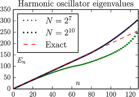
Figure 1. The 128 lowest eigenvalues of Equation (15), computed with the standard 3-stensil approximation for the Laplace operator (here the kinetic energy T). The parameters are chosen to illustrate two typical effects: With the bc = (a, a) boundary conditions the harmonic oscillator potential is effectively changed to V = ∞ for x ≥ 12.5, thereby modifying the behavior of extended (highly exited) states. The effect of this is to increase the eigenenergies of such states, to a behavior more similar to a particle-in-box. This is visible for n ≳ 80. The effect of using the 3-stensil approximation for T is to change the spectrum of this operator from k2 to (the slower rising) (2/δx)2sin2(kδx/2). This is visible in the sub-linear rise of the spectrum for N = 27.
For a better quantitative assessment of the accuracy obtained we plot some energy differences, , in Figure 2.
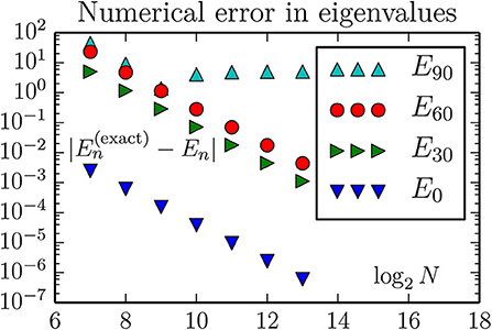
Figure 2. The discretizations error of energy eigenvalues when using the standard 3-stensil approximation for the one-dimensional Laplace operator (here the kinetic energy T). There is no improvement in E90 beyond a certain lattice size N, because the corresponding oscillator state is too large for the geometric region. Hence, for improved accuracy of higher eigenvalues one should instead increase the xe, while maintaining xo = −xe/2. For the other states the improvement is consistent with the expectation of an error proportional to δx2. This predicts an accuracy improvement of magnitude 212 = 4, 096 when the number of lattice sites increases from N = 27 to N = 213 for a fixed geometry. The eigenvalues are computed by the dense matrix routine eigvalsh from scipy.linalg.
This brute force method leads to a dramatic increase in memory requirement with increasing lattice size. For a lattice with N = 2m sites, the matrix requires storage of 4m double precision (8 byte) numbers. For m = 13 this corresponds to about of memory, for m = 14 about 2Gb. The situation becomes even worse in higher dimensions.
Assuming that we are only interested some of the lowest eigenvalues, an alternative approach is to calculate these by the iterative routine eigsh from scipy.sparse.linalg. This allows extension to larger lattices, as shown in Figure 3.
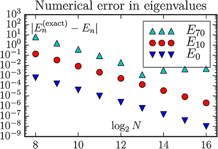
Figure 3. The discretizations error computed by the routine eigsh from scipy.sparse.linalg. For a fixed lattice size the discretizations error is essentially the same as with dense matrix routines. However, with a memory requirement proportional to the lattice size (instead of its square) it becomes possible to go to much larger lattices. This figure also demonstrates (E70) that the error can be limited by boundary effects instead of the finite discretization length δx.
With a sparse eigenvalue solver the calculation becomes limited by available computation time, which in many cases is a much weaker constraint: With proper planning and organization of calculations, the relevant timescale is the time to analyze and publish results (i.e., weeks or months). The computation time is nevertheless of interest (it shouldn't be years). We have measured the wall clock time used to perform the computations for Figures 2, 3, performed on a 2012 Mac Mini with 16 Gb of memory, and equipped with a parallelized scipy library. Hence, the eigvalsh and eigsh routines are running with four threads. The results are plotted in Figure 4.
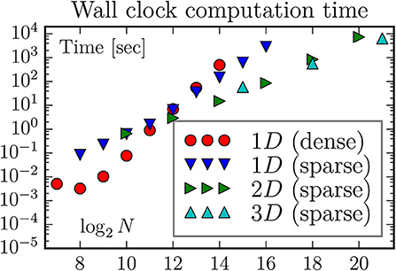
Figure 4. The wall clock time used to find the lowest 128 eigenvalues, for various systems and methods. We have also used the dense matrix routine eigvalsh to compute the eigenvalues of a 27 × 27 (N = 214) two-dimensional lattice; not unexpected it takes the same time as for a 214 one-dimensional lattice. Somewhat surprisingly, with eigsh it is much faster to find the eigenvalues for two-dimensional lattice than for a one-dimensional with the same number of sites, and somewhat faster to find the eigenvalues for a three-dimensional lattice than for the two-dimensional with the same number of sites.
Here we have used the eigsh routine in the most straightforward manner, using default settings for most parameters. This means, in particular, that the initial vector for the iteration (and the subsequent set of trial vectors) may not be chosen in a optimal manner for our category of problems. It is interesting to observe that eigsh works better for higher-dimensional problems. The (brief) scipy documentation [17] says that the underlying routines works best when computing eigenvalues of largest magnitude, which are of no physical interest for our type of problems. It is our experience that the suggested strategy, of using the shift-invert mode instead, does not work right out-of-the-box for problems of interesting size (i.e., where dense solvers cannot be used). We were somewhat surprised to observe that the computation time may decrease if the number of computed eigenvalues increases (cf. Figure 5).
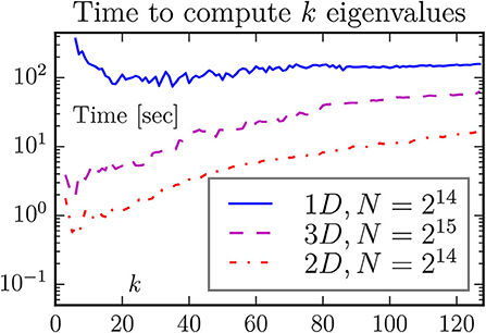
Figure 5. One may think that it takes longer to compute more eigenvalues. This is not always the case when the number of eigenvalues is small, as demonstrated by this figure. The default choice of eigsh is to compute k = 6 eigenvalues. For our two- and three-dimensional problems this looks close to the optimal value, but it is too low for the one-dimensional problem.
4.2. Example: 2- and 3-Dimensional Harmonic Oscillators
The d-dimensional harmonic oscillator
has eigenvalues En = (d + 2n), for n = 0, 1, …. The degeneracy of the energy level En is gn = (n + 1) in two dimensions, and in three dimensions1. This degeneracy may be significantly broken by the numerical approximation. For a numerical solution we only have to change the previous parameters slightly:
for dim = 2, 3.
As already discussed, the routine eigsh works somewhat faster in higher dimensions than in one dimension (for the same total number N of lattice points). The corresponding discretizations errors are shown in Figures 6, 7.
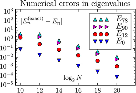
Figure 6. The discretization error of energy eigenvalues when using the standard 5-stensil approximation for the two-dimensional Laplace operator. Exactly, the states E78 and E90 are the two edges of a 13-member multiplet with energy 26, and the state E12 is the middle member of a 5-member multiplet with energy 10. With the chosen parameters all states considered a well confined inside the geometric region; hence we do not observe any boundary correction effects.
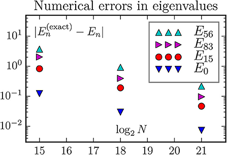
Figure 7. The discretization error of energy eigenvalues when using the standard 7-stensil approximation for the three-dimensional Laplace operator. Exactly, the states E56 and E83 are the two edges of a 28-member multiplet with energy 15, and the state E15 is the middle member of a 10-member multiplet with energy 9.
The discretizations error continues to scale like δx2. This means that a reduction of this error by a factor 22 = 4 requires an increase in the number of lattice points by a factor 2d in d dimensions. This means that is becomes more urgent to use a better representation of the Laplace operator in higher dimensions. Fortunately, as we shall see in the next sections, better representations are available for our type of problems.
5. FFT Calculation of the Laplace Operator
One improvement is to use the reflection symmetry of each axis (x → −x, y → −y, etc.) to reduce the size of the spatial domain. This reduces δx by a half, without changing the number of lattice points.
A much more dramatic improvement is to use some variant of a Fast Fourier Transform (FFT): After a Fourier transformation, , the Laplace operator turns into multiplication operator,
This means that application of the Laplace operator can be represented by (i) a Fourier transform, followed by (ii) multiplication by k2, and finally (iii) an inverse Fourier transform. Essentially the same procedure works for the related trigonometric transforms.
For rectangular lattices, these options can also be implemented as practical procedures, due to the existence of efficient and accurate2 algorithms for discrete Fourier and trigonometric transforms. The time to perform the above procedure is not very much longer than the corresponding stensil operations. The benefit is that the Laplace operator becomes exact on the space of functions which can be represented by the modes included in the discrete transform.
We have coded this FFT-type representation of the Laplace operator for the various types of boundary conditions listed in Table 1. This possibility can be chosen as an option for the kinetic energy selector, ke. The obtainable accuracy through this option increases dramatically, as illustrated in Figures 8–11. As shown in Figure 8, a decrease of the lattice length δx does not necessarily lead to a more accurate result. We attribute this to an enhanced amplification of roundoff errors.
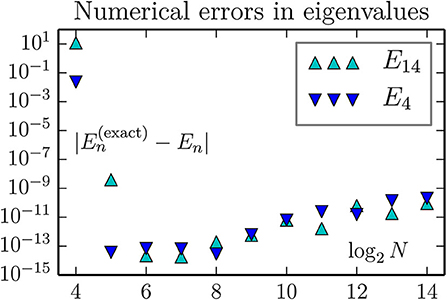
Figure 8. With a FFT representation of the Laplace operator the discretization error drops exceptionally fast with δx∝N−1. When it becomes “small enough” the effect of numerical roundoff becomes visible; the latter leads to an increase in error with δx. The results in this figure is for a one-dimensional lattice, but the behavior is the same in all dimensions. The lesson is that we should make δx “small enough” (which in general may be difficult to determine a priori), but not smaller. It may also be possible to rewrite the eigenvalue problem to a form with less amplification of roundoff errors.
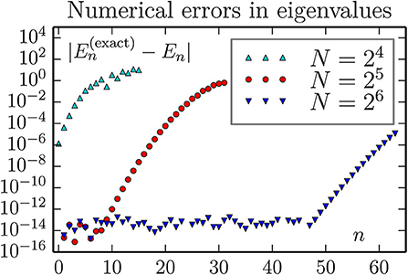
Figure 9. Accuracy of computed eigenvalues for a 1D oscillator, using the FFT approximation for kinetic energy T. This figure may suggest that an increase in the number of lattice size N will lead to a accurate treatment of states with higher n. Our findings are that this is not the case: The results for N = 27 and N = 28 have essentially the same behavior as for N = 26.
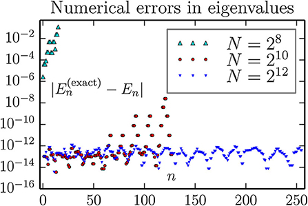
Figure 10. Accuracy of computed eigenvalues for a 2D oscillator, using the FFT approximation for kinetic energy T. As can be seen, a large number of the lowest eigenvalues can be computed to an absolute accuracy in the range 10−14–10−12 with a lattice of size 26 × 26. We observe not improvement by going to 27 × 27 lattice, but no harm either (except for an increase in the wall clock execution time from about 3 to 30 s for each combination of boundary conditions).
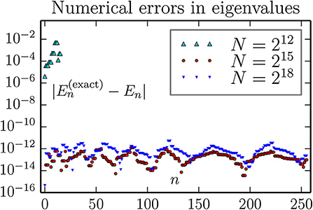
Figure 11. Accuracy of computed eigenvalues for a 3D oscillator, using the FFT approximation for kinetic energy T. As can be seen, a large number of the lowest eigenvalues can be computed to an absolute accuracy in the range 10−14 to 10−12 with lattice of size 26 × 26 × 26. We observe no improvement by going to 27 × 27 × 27 lattice, but no harm either (except for an increase in the wall clock execution time from about 6 to 95 min for each combination of boundary conditions).
It might be that the harmonic oscillator systems are particularly favorable for application of the FFT representation. One important feature is that the Fourier components of the harmonic oscillator wave functions vanishes exponentially fast, like e−k2/2, with increasing wave-numbers k2. This feature is shared with all eigenfunctions of polynomial potential Schrödinger equations, but usually with different powers of k in the exponent, which quantitatively leads to a somewhat different behavior. Furthermore, the onset of exponential decay will occur for larger values of k2 for the more excited states (i.e., with larger eigenvalue numbers).
For systems with singular wavefunctions the corresponding Fourier components may vanish only algebraically with k2. An equally dramatic increase in accuracy cannot be expected for such cases.
6. Anharmonic Oscillators
Our general setup allows for any computable potential, by simply changing the definition of the function assigned to V (This does not mean that every potential will lead to a successful calculation of eigenvalues). For demonstration and comparison purposes, like here, one encounters the problem that the exact answers are no longer known. This makes it more difficult to assess the accuracy and other qualities of the code. As an example where some instructive comparisons are possible, we consider the two-dimensional anharmonic oscillator obeying the Schrödinger equation,
By construction, this problem has separable solutions of the form
where the factors ψ obey a one-dimensional equation,
and E = εm + εn. As mentioned in the introduction, equations like the latter have been quite intensely studied in the literature. Accurate values for the even parity eigenvalues of Equation (20) can for instance be found in Table 1 of [9]. In Table 2, we list the 10 lowest eigenvalues to 30 decimals precision, calculated by the very-high-precision method described in [14]. Hence, for practical purposes all εm of interest can be considered exactly known. This means that the eigenvalues E of Equation (18) can also be considered exactly known. We list the 22 lowest ones of them in Table 3. These are the values we want to compare against the standard solution methods. The latter make no use of the separability property of the problem, which anyway is destroyed by the lattice approximation.
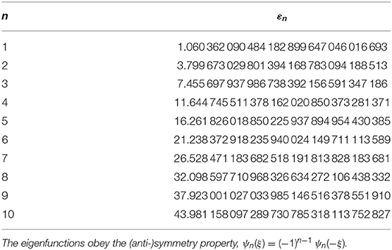
Table 2. The 10 lowest eigenvalues of the quantum anharmonic oscillator, calculated to high precision by the method described in [14], from the Schrödinger equation .
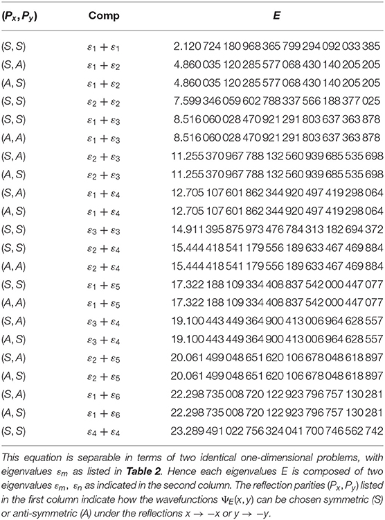
Table 3. The 22 lowest eigenvalues E of the two-dimensional quantum anharmonic oscillator, as defined by the Schrödinger equation displayed to 30 decimals accuracy.
The first column of Table 3 associates a symmetry classification (Px, Py) to each eigenvalue E, or rather to its corresponding eigenfunction ΨE(x, y). Since Equation (18) are invariant under reflections,
all eigenfunctions can be constructed to transform symmetrically (S) or anti-symmetrically (A) under such reflections. For m < n, such a construction is
For m = n there is only one possibility,
By use of the properties that
we find that
and further that Ψmm(−x, y) = Ψmm(x, − y) = Ψmm(x, y). The conclusion is that in an exact calculation the states Ψmn will be double degenerate when m ≠ n, with parities (Px, Py) equal to (S, S) and (A, A) when m, n are both even or both odd, otherwise with parities (S, A) and (A, S). The states Ψmm are singlets with parities (S, S). The first column of Table 3 is constructed according to these rules.
Table 4 displays the results of some standard numerical solutions to Equation (18), “automagically” generated in the same way as the previous treatments of the harmonic (linear) oscillators. In the second column we show the results of using the minimal 5-point stensil approximation of the Laplace operator on a 1, 024 × 1, 024 lattice (approximating the whole space). The resulting numerical problem is solved with the eigsh sparse solver. The numerical accuracy is indicated by an underscore of the first inaccurate position, when taking proper roundoffs into account: The exact and numerical results are rounded off to the same number of digits, and compared; the underscore indicates the first position where the results differ.
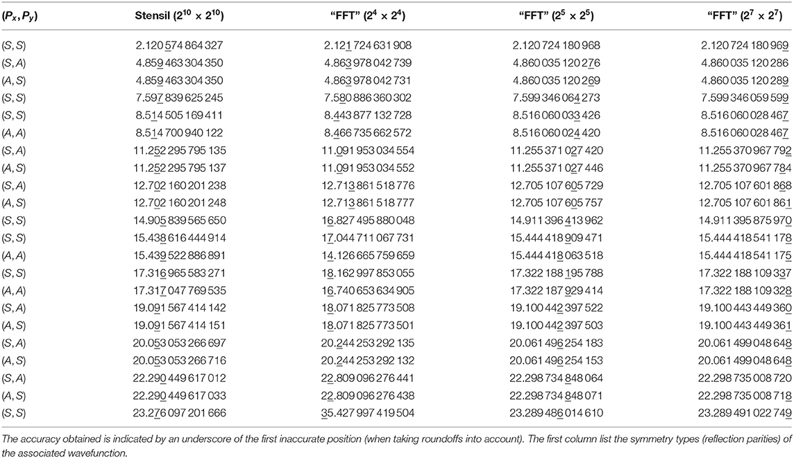
Table 4. Numerical calculations of the lowest eigenvalues of the two-dimensional quantum anharmonic oscillator, by various approximations and lattice sizes.
As can be seen, the results are less than impressive, taking into account the amount computational work invested. One straightforward improvement is to utilize the reflection symmetries of the problem to reduce the magnitude of the problem (with the same lattice cell size δx2) by a factor 4, or to reduce the lattice cell size δx2 (with the same problem magnitude) by a factor 4. Another option is to use a higher order stensil approximation like (13). However, as already discussed in section 5, an even better option (for this class of problems) is to use a FFT type of approximation of the Laplace operator. The resulting eigenvalues are listed in columns 3–5, for various lattice sizes approximating the upper right quadrant (x ≥ 0, y ≥ 0) of space. For each lattice size the problem must be solved 4 times, with symmetric (S) and anti-symmetric (A) boundary conditions at the axes x = 0 and y = 0.
By symmetry under interchange, x ↔ y, we expect the (S, A) and (A, S) to give identical results (as long as the lattice approximation respects this symmetry). As can be seen, the numerical results satisfy the symmetry within a numerical accuracy of few × 10−12, regardless how close the results are to the exact values. The degeneracy of states with (S, S), respectively, (A, A) symmetry cannot be deduced in the same way from the lattice approximated problem. In the infinite space formulation the problem is separable, which in turn implies this degeneracy. However, the lattice approximation introduces boundaries that are non-factorizable in the (ξ, η)-coordinates. This means that the problem is no longer separable in the lattice approximation. As a result the degeneracy of the (S, S) and (A, A) energies are split by a much larger amount, of the same order as the difference between exact and numerical results. (In this case, the lattice problem could be made separable by a rotation of the lattice orientation by 45 degrees.)
We observe that even a 24 × 24 lattice with in the “FFT approximated” Laplace operator provide almost equally accurate results as a 210 × 210 lattice with the 5-stensil approximation. The results from a 25 × 25 lattice seems more than sufficient for practical purposes (say compared to experimental obtainable accuracy), with little to be gained by further decrease of the lattice length δx.
The computation times for the “FFT approximation” are about 0.06, 0.8, and 75 s for respectively 16 × 16, 32 × 32, and 128 × 128 lattice sizes. For the same number of lattice points, the 5-stensil formulation may lead to somewhat shorter computation times. But this is completely offset by the need to work with a much larger number of lattice points: The computation time for the 1, 024 × 1, 024 stensil approximation was about 30 min.
The Python package described in this paper is available at [19].
Data Availability Statement
The raw data [19] supporting the conclusions of this article will be made available by the authors, without undue reservation.
Author Contributions
All authors listed have made a substantial, direct and intellectual contribution to the work, and approved it for publication.
Conflict of Interest
The authors declare that the research was conducted in the absence of any commercial or financial relationships that could be construed as a potential conflict of interest.
Acknowledgments
An early version of this work was presented at the IAENG International MultiConference of Engineers and Computer Scientists, Hong Kong March 18–20, 2015, as documented in [20].
AM would like to thank Mathematics Teaching and Learning Research Group within The department of mathematics, Bodø, Nord University for partial support.
Footnotes
1. ^The general formula is .
2. ^The error of a back-and-forth FFT is a few times the numerical accuracy, i.e., in the range 10−14 to 10−15. with double precision numbers. However, when an error of this order is multiplied by k2 it can be amplified by several orders of magnitude. Hence, the range of k2-values should not be chosen significantly larger than required to represent ψ(r) to sufficient accuracy.
References
1. Dirac PAM. The fundamental equations of quantum mechanics. Proc R Soc A. (1925) 109:642–53. doi: 10.1098/rspa.1925.0150
2. Schrödinger E. An undulatory theory of the mechanics of atoms and molecules. Phys Rev. (1926) 28:1049–70. doi: 10.1103/PhysRev.28.1049
3. Pauli W. Über die Wasserstoffspektrum vom Standpunkt der neuen Quantenmechanik. Zeitsch Phys. (1926) 36:336–63.
4. Heisenberg W. Über quantentheoretische Umdeutung kinematischer und mechanischer Beziehungen [Quantum-theoretical reinterpretation of kinematic and mechanical relations]. Zeitsch Phys. (1925) 33:879–93.
5. Bender CM, Wu TT. Analytic structure of energy levels in a field-theory model. Phys Rev Lett. (1968) 21:406–9. doi: 10.1103/PhysRevLett.21.406
6. Bender CM, Wu TT. Anharmonic oscillator. Phys Rev. (1969) 184:1231–60. doi: 10.1103/PhysRev.184.1231
7. Bender CM, Wu TT. Large-order behavior of perturbation theory. Phys Rev Lett. (1971) 27:461–5. doi: 10.1103/PhysRevLett.27.461
8. Bender CM, Wu TT. Anharmonic oscillator. II. A study of perturbation theory in large order. Phys Rev D. (1973) 7:1620–36. doi: 10.1103/PhysRevD.7.1620
9. Bender CM, Olaussen K, Wang PS. Numerological analysis of the WKB approximation in large order. Phys Rev D. (1977) 16:1740–8. doi: 10.1103/PhysRevD.16.1740
10. Zinn-Justin J, Jentschura UD. Multi-instantons and exact results I: conjectures, WKB expansions, and instanton interactions. Ann Phys. (2004) 313:197–267. doi: 10.1016/j.aop.2004.04.004
11. Zinn-Justin J, Jentschura UD. Multi-instantons and exact results II: specific cases, higher-order effects, and numerical calculations. Ann Phys. (2004) 313:269–325. doi: 10.1016/j.aop.2004.04.003
12. Noreen A, Olaussen K. Quantum loop expansion to high orders, extended borel summation, and comparison with exact results. Phys Rev Lett. (2013) 111:040402. doi: 10.1103/PhysRevLett.111.040402
13. Janke W, Kleinert H. Convergent strong-coupling expansions from divergent weak-coupling perturbation theory. Phys Rev Lett. (1995) 75:2787–91. doi: 10.1103/PhysRevLett.75.2787
14. Mushtaq A, Noreen A, Olaussen K, Øverbø I. Very-high-precision solutions of a class of Schrödinger type equations. Comput Phys Commun. (2011) 182:1810–3. doi: 10.1016/j.cpc.2010.12.046
15. Noreen A, Olaussen K. High precision series solutions of differential equations: ordinary and regular singular points of second order ODE's. Comput Phys Commun. (2012) 183:2291–7. doi: 10.1016/j.cpc.2012.05.015
16. Van Der Walt S, Colbert SC, Varoquaux G. The NumPy array: a structure for efficient numerical computation. Comput Sci Eng. (2011) 13:22–30. doi: 10.1109/MCSE.2011.37
17. Jones E, Oliphant T, Peterson P. SciPy: Open Source Scientific Tools for Python. (2014). Available online at: http://www.scipy.org/
18. Oliphant TE. Python for scientific computing. Comput Sci Eng. (2007) 9:10–20. doi: 10.1109/MCSE.2007.58
19. Mushtaq A, Noreen A, Olaussen A. Python Package for Numerical Solutions of Quantum Mechanical Eigenvalue Problems (2020). doi: 10.6084/m9.figshare.127655
Keywords: numpy array, FFT (fast fourier transform), quantum mechanics, python classes, eigenvalue problems, sparse SciPy routines, Schrödinger equations
Citation: Mushtaq A, Noreen A and Olaussen K (2020) Numerical Solutions of Quantum Mechanical Eigenvalue Problems. Front. Phys. 8:390. doi: 10.3389/fphy.2020.00390
Received: 30 November 2019; Accepted: 11 August 2020;
Published: 28 September 2020.
Edited by:
Jesus Martin-Vaquero, University of Salamanca, SpainReviewed by:
Kazuharu Bamba, Fukushima University, JapanJan Sladkowski, University of Silesia of Katowice, Poland
Copyright © 2020 Mushtaq, Noreen and Olaussen. This is an open-access article distributed under the terms of the Creative Commons Attribution License (CC BY). The use, distribution or reproduction in other forums is permitted, provided the original author(s) and the copyright owner(s) are credited and that the original publication in this journal is cited, in accordance with accepted academic practice. No use, distribution or reproduction is permitted which does not comply with these terms.
*Correspondence: Asif Mushtaq, YXNpZi5tdXNodGFxQG5vcmQubm8=