Toward interpretable expected goals modeling using Bayesian mixed models

Empowered by technological progress, sports teams and bookmakers strive to understand relationships between player and team activity and match outcomes. For this purpose, the probability of an event to succeed (e.g., the probability of a goal to be scored, namely, xG for eXpected Goals) provides insightful information on team and player performance and helps statistical and machine learning approaches predict match outcomes. However, recent approaches require powerful but complex models that need more inherent interpretability for practitioners. This study uses a Bayesian generalized linear mixed-effects model to introduce a simple and interpretable xG modeling approach. The model provided similar performance when compared to the StatsBomb model (property of the StatsBomb company) using only seven variables relating to shot type and position, and surrounding opponents (AUC = 0.781 and 0.801, respectively). Pre-trained models through transfer learning are suitable for identifying teams’ strengths and weaknesses using small sample sizes and enable interpretation of the model’s predictions.

1 Introduction

Football is a globally popular sport and its financial and social impact attracts researchers whose main aim is to increase comprehension of training and match-play performance (1–3). Thanks to technological and analytical evolutions, new performance-oriented research perspectives have emerged from the analysis of player performance. Both training and match data, collected from football players using global navigation satellite systems (4) and markerless optical tracking systems (5), have become more plentiful and increasingly accurate. The information enables the development of advanced statistical and machine learning approaches to help analyze and subsequently optimize football performance and attempt predictions of match outcomes.

A popular performance metric in football is expected goals (xG). This metric represents the probability of a shot resulting in a goal. It was first introduced in football by Green (6) with the aim of identifying the key factors underpinning how goals are scored and has become a valuable objective measure of an individual player’s performance that can also be extended to the team level (7–10). To date, xG models typically account for spatio-temporal information, such as the time, the distance and angle between the player and the goal at the shooting time, the type of shot, and the preceding event (i.e., the last action such as a low pass or a high pass). Beyond these data, previous studies have reported different approaches and model architectures (11–16). Modeling xG requires multiple features as the complexity of the task and its variability calls into question its predictability when using a restricted set of game features (e.g., the goal distance) (15). However, Umami et al. (16) reported that a logistic regression using only a few features (the distance and angle to the goal, and whether the shot is headed or not) provided convincing results. Alternatively, more complex architectures have been employed to attempt to better estimate xG (14). In effect, the authors in the latter study compared a logistic regression with non-linear ensemble learning algorithms (random forest and adaptive boosting) to predict the match score by summing the estimated xG of each shot opportunity. According to their results, the random forest algorithm provided the best model performance. In another study, Anzer and Bauer (11) used advanced features such as the height of the ball when the shot was attempted and analysis of the player’s movement at the time of the shot. By comparing several supervised machine learning models, a gradient boosting model that accounted for the type of shot (header, leg kick, and direct free kick) provided the best performance in predicting the number of goals scored.

Most studies that have attempted to model xG have focused on fitting the best model using non-linear and complex model architectures, at the expense of model interpretability. These studies aimed to achieve the best performance in predicting that the shot will be converted into a goal. However, complex models are difficult to interpret. There are methods for explaining such models, such as the use of Shapley values (17, 18), but these approaches are still criticized today (19, 20), questioning the ability of one to fully master the complexity of Shapley value calculations. There are a few studies that have focused on xG modeling while preserving interpretability. To build a model that identifies key factors influencing xG, Decroos and Davis (13) and Bransen and Davis (12) proposed the use of a generalized additive model (GAM). The studies show that GAMs provide comparable results to a more complex gradient boosting model while retaining the advantage of interpretability. To further improve the interpretability of the model and since logistic regression has proved effective in modeling xG (16), one should consider the relationships between features and xG to be linear and consequently should utilize a generalized linear model instead of a GAM. One also assumes that soccer games evolve and that patterns are slightly different across seasons and competitions. As such, the present authors made a choice to investigate a Bayesian framework with mixed effects. Very recently, Scholtes and Karakuş (21) also proposed a hierarchical Bayesian approach to model xG. They used this model to determine whether the individual player or their positional role impacted xG. The main strength of their work was the identification of specific player abilities throughout an interpretable model and a rigorous assessment of prediction uncertainty. However, the potential of the Bayesian framework was arguably not fully exploited and further research is warranted.

In the present article, an alternative prior specification method is proposed to model xG: an interpretable Bayesian generalized linear mixed-effects model (22). This model might achieve better estimation quality, and its benefits are potentially numerous. First, the linear structure makes the model very easy to interpret by analyzing the model’s coefficients. Second, the inclusion of random effects means that intra- and inter-player/team variability can be considered. This enables interpretation of the strength of players and/or teams in specific game situations. Third, using the Bayesian framework enables the utilization of limited training data while incorporating expert prior knowledge. Such a model is not new and is used in other fields and applications. Yet, it was unseen in xG modeling until the recent work of Scholtes and Karakuş (21) and also demonstrates the aforementioned advantages. In our study, we propose to further exploit the Bayesian contribution with a transfer learning strategy to build a highly informative prior. The prior is built using past competition, rather than relying on a hand-constructed prior, which is inevitably less informative. A study on the impact of prior choice on the posterior was presented using the Wasserstein Impact Measure (WIM) (23), showing the benefits of choosing the prior we propose (more informative prior and better predictive performance). Furthermore, a practical model explainability of outcomes is provided through Shapley Additive exPlanations estimates (SHAP), which can, according to the literature (24), benefit football analysts and coaches in their decision-making processes.

Following the presentation of the data and the features used to evaluate xG (Section 2.1), we will define our xG model (Section 2.2) and then present the results (Section 3). Thereafter, we will engage in a discussion of the results and benefits of the model within the context of the existing literature (Section 4).

2 Material and methods

2.1 Dataset description

Here, we used the StatsBomb open dataset (25) that includes 460 matches with 63,177 shots from 11 different competitions including the FIFA World Cup, Women’s World Cup, UEFA Euro, UEFA Women’s Euro, Indian Super League, NWSL, and Premier League between 2003 and 2022. Among these shots, we retained 59,417 from open-play situations and discarded 3,760 from set-play actions (penalty, free kick, or corner). Hence, only shots from open play were considered. Shot location and occurrence is displayed in Figure 1.

Figure 1

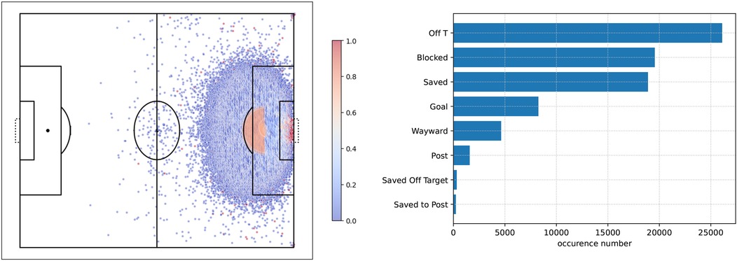
Figure 1. Shot outcomes. On the left, dots represent shot locations on the field and the gradient color denotes the frequency of scored shots per location. On the right, all outcomes and their occurrences are listed.

Shot data include the ball’s location, the player’s location, and the time of the shot. From these spatio-temporal data, we extracted features for subsequent modeling. An exhaustive list of the features is provided in Table 1. Many of these features are well-known and are common to previous studies (11, 26). However, subtle features such as the Best_angle may provide relevant information. Since our dataset includes quantitative and qualitative features (Position, Body_part, and Last_action), the latter have been one-hot encoded for the modeling. To reduce dimensionality and prevent collinearity, we performed a feature selection as described in Section 2.2.

Table 1

Table 1. Feature descriptions and value range.

The StatsBomb dataset provides an estimate of xG, which we will refer to as StatsBomb xG. Their model, which remains undetailed, has most likely been trained on their full dataset of matches instead of the open-source dataset used in our study. Furthermore, some features such as shot impact height are used and not shared in the open-source data set. This StatsBomb xG estimate, which has proven its performance (27, 28), will be considered as a baseline model for comparison.

2.2 Model definition

In the literature, many statistical and machine learning methods have been tested to model xG (presented in Section 1), most of them focusing on the best predictive performance at the expense of model interpretability. In this study, we propose a model allowing a detailed analysis of the shot quality. We built a Bayesian logistic regression with mixed effects, defined in Equations 1 and 2. Normal and Gamma prior distributions (see Equation 3) have been set for fixed and random effects, with adjusted means and standard deviations accordingly (the method is described hereafter).

Let us define ${\mathit{x}}_i$ and $y_i$, respectively, as the vector of feature values and the shot result for observation $i$ ($y_i\in \{0,1\}$, $1$ represents a goal and $0$ otherwise). Hence, we define $y_{i_k}$ such that the $i$ predicted xG for a team $k$ in the following:

$y_{i_k}=(1+e^{-{\theta }_{i_k}}{)}^{-1}+{ϵ}_{i_k},{ϵ}_{i_k}\sim \mathcal{N}(0,{\sigma }_i^2),(1)$

${\theta }_{i_k}=\alpha +\sum _{j=1}^p({\beta }_j+{\eta }_i^{({\beta }_j)})x_{i_{k}j}+{\eta }_i^{(\alpha )},{\eta }_i^{(q)}\sim \mathcal{N}(0,{\omega }_q^2),(2)$

$\begin{array}{rl}\alpha & \sim \mathcal{N}({\mu }_{\alpha },{\sigma }_{\alpha }^2),\mathit{\beta }\sim \mathcal{N}({\mathit{\mu }}_{\beta },{\mathbf{\Sigma }}_{\beta }),{\omega }_q\sim \mathrm{\Gamma }(a_q,b_q),\\ \sigma & \sim \mathrm{\Gamma }(a,b)\end{array}.(3)$

where $q\in \{\alpha ,{\beta }_1,\dots ,{\beta }_p\}$ are the fixed effects parameters to be identified, $p$ is the number of features, $i\in \{1,\dots ,N\},k\in \{1,\dots ,n_i\}$, $N$ is the number of teams, and $n_i$ is the number of observations for team $i$. Moreover, the parameters $q\in \{\alpha ,{\beta }_1,\dots ,{\beta }_p\}$ on which random effects ${\eta }_i^{(q)}$ are applied must be determined. The model selection is performed using Pareto-smoothed importance sampling-leave-one-out (PSIS-LOO) (29). This Bayesian approach to model selection enables us to select the model that offers the best predictive accuracy in a robust way thanks to its leave-one-out strategy. In addition, the combination of Hamiltonian Monte Carlo and approximate cross-validation enables highly efficient model fitting and score estimation for a wide range of model selection contexts (30). Thus, not all ${\eta }_i^{(q)}$ will be considered a random variable but some will be fixed to 0.

The choice of the prior distribution is a crucial step in the model fitting process (choice of ${\mu }_{\alpha },{\sigma }_{\alpha },{\mathit{\mu }}_{\beta },{\mathbf{\Sigma }}_{\beta },a_q,b_q,a,b$). Alternatively, two different approaches can be considered instead of a non-informative prior, with (i) a prior identification from expert knowledge, and (ii) a prior identification using a baseline model, computed on different data. Scholtes and Karakuş (21) used the first method while the latter method has been employed in this study, thus considering a different training dataset. Hence, estimating prior distributions using a separate dataset ensures unbiased model training and model generalization. Our method therefore uses a transfer learning strategy (i.e., the reuse of a set of functions or knowledge learned from a source task). A model is fitted for each competition, the prior being built from the other competitions. In other words, let us assume that $c$ is the competition of interest and that $\overline{c}$ are the other competitions available in our dataset. The $\overline{c}$ are used to fit a model $\mathcal{M}$ without informative prior knowledge. The model of interest, fitted on $c$, then benefits from the posterior knowledge identified in $\mathcal{M}$.

A Bayesian model with flat prior and without random effect was fitted on the shots from $\overline{c}$. The posterior distribution obtained is then used to build the prior for the model on competition $c$, and is defined as

$\alpha \sim \mathcal{N}({\hat{\alpha }}_{\overline{c}},g.{\hat{\sigma }}_{{\alpha }_{\overline{c}}}^2),\mathit{\beta }\sim \mathcal{N}({\hat{\mathit{\beta }}}_{\overline{c}},g.{\hat{\mathbf{\Sigma }}}_{{\beta }_{\overline{c}}}).$

The coefficient $g$ is chosen so that the mean of the standard deviations for the fixed effects is equal to $0.5$ to ensure that the prior information is neither too strong nor too weak. Regarding the parameters $\sigma$ and ${\omega }_q,q\in \{\alpha ,{\beta }_1,\dots ,{\beta }_p\}$, the priors were fixed to $\sigma \sim \mathrm{\Gamma }(1,0.5),{\omega }_q\sim \mathrm{\Gamma }(0.3,0.1)$. The variance of $\sigma$ prior distribution is large, while ${\omega }_q,q\in \{\alpha ,{\beta }_1,\dots ,{\beta }_p\}$ is more restrictive. This allows us to avoid the high values obtained when teams are under-represented in the studied competition, and when observations are not necessarily representative of actual team performance.

Posterior distributions have been estimated through Markov chain Monte Carlo with a Hamiltonian Monte Carlo algorithm [No-U-Turn Sampler, (31)]. The No-U-Turn sampler allows us to simplify the tuning of the standard Hamiltonian Monte Carlo method with a similar efficient performance. Then, on the basis of the sampling obtained, we used 10,000 iterations and four chains, with a burn-in period of 1,000 samples for sampling. All the analyses were conducted using the latest version of the Python library PyMC (32). Once the sampling from the posterior distribution was complete, the model’s parameters were estimated according to the maximum a posteriori for further predictions.

For a given competition, 70% of the shots were used as a training set while the remaining 30% were used as a test set. All the results presented in Section 3 stem from the test set. Model selection was carried out using PSIS-LOO for each competition to select $q$ parameters on which random effects are applied. Consequently, the random effect structure could vary across competitions.

As the work of Scholtes and Karakuş (21) is analogous to ours, we also fitted their model to our data and features (selected in Section 2.3) to emphasize the benefits of using an informative prior in small datasets. The following priors presented in this section correspond to the priors used to reproduce their work. The same features used to fit our model were considered, but the priors were chosen as proposed in their paper. Since some features are shared between our respective works, the priors chosen for the associated parameters are the identical ($\mathcal{N}$ stands for normal distribution and $\mathcal{S}\mathcal{N}$ for skew-normal distribution):

• $intercept$ : $\mathcal{N}(\mu =0,\sigma =5)$

• $distance\mathrm{\_}goalkeeper$ : $\mathcal{N}(\mu =0,\sigma =5)$

• $distance$ : $\mathcal{S}\mathcal{N}(\mu =-1,\sigma =5,\alpha =-1)$

• $body\mathrm{\_}part\mathrm{\_}head$ : $\mathcal{N}(\mu =0,\sigma =5)$

• $nb\mathrm{\_}opponent\mathrm{\_}traj$ : $\mathcal{S}\mathcal{N}(\mu =-1,\sigma =5,\alpha =-1)$

For the other features, we applied the same method for their selection and finally used the following priors:

• $best\mathrm{\_}angle$ : $\mathcal{S}\mathcal{N}(\mu =1,\sigma =5,\alpha =1)$This feature is similar to the shot_angle feature used in Scholtes and Karakus’ paper, which is the left post, shot location, and right post angle. The prior is therefore the same as that used in their article for the shot_angle feature.

• $angle$ : $\mathcal{S}\mathcal{N}(\mu =-1,\sigma =5,\alpha =-1)$The angle we use represents alignment with the goal. A higher value represents a less centered positioning, which translates into a lower score probability and explains the choice of $\mu$ and $\alpha$.

• $closest\mathrm{\_}opponent$ : $\mathcal{S}\mathcal{N}(\mu =1,\sigma =5,\alpha =1)$$\mu =1$ and $\alpha =1$ because the closer the opponent, the greater the pressure.

In the following, we will refer to this model as Scholtes’ model.

2.3 Feature selection and performance criteria

To use our approach, the model used to build the prior must be fitted using the same features as the model of interest. Thus, feature selection was conducted using the training set of all competitions in a global model. A frequentist logistic regression was performed, discarding random effects and any prior knowledge. For feature selection, we performed a forward selection starting with the best features to model xG and then added features one by one until the area under the curve (AUC) reached a plateau (see Figure 2). At each step, all unused features were tested.

Figure 2

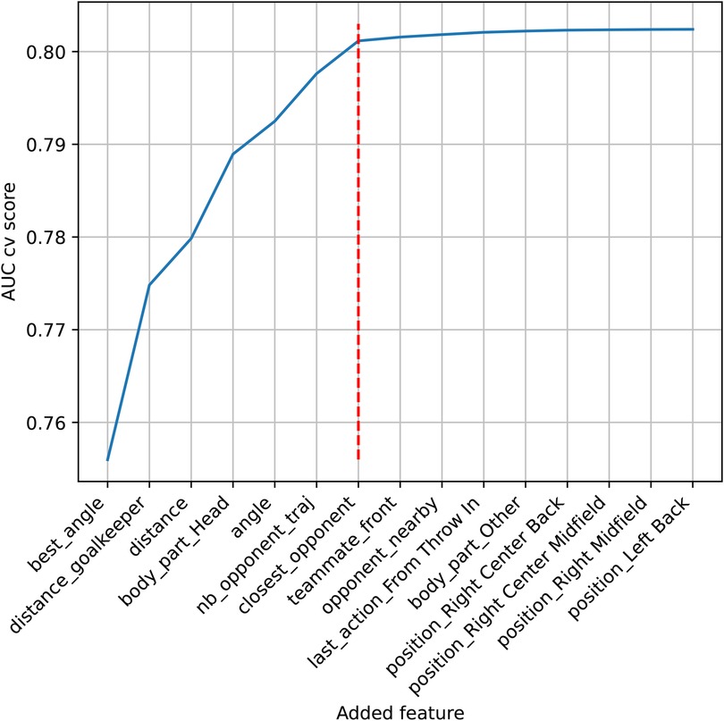
Figure 2. AUC score evolution of the fivefold cross-validation. On the x-axis, the best features are added one by one. The red dotted line represents the last selected feature, where the AUC reaches a plateau.

Seven features were selected from the fivefold cross-validation (Figure 2), with (1) best_angle, (2) distance_goalkeeper, (3) distance, (4) body_part_head (one-hot-encoded feature, $1$ if the shooter struck the ball with their head, $0$ otherwise), (5) angle, (6) nb_opponent_traj, and (7) closest_opponent. They constitute the set of predictors for subsequent modeling.

The area under the curve, balanced accuracy, precision, recall, specificity, and F1 score were used to measure the efficiency of the models.

Each competition was used for model fitting, leading to models with heterogeneous fixed parameter estimates based on the prior information.

3 Results

The comparison of the performance of the proposed model (i.e., a Bayesian mixed effect logistic regression, namely, Bayesian xG) with that of StatsBomb’s and Scholtes’ models is reported in Table 2. Considering all competitions, the results show that model performances differed slightly, but similar performance was obtained with the Bayesian approach and the StatsBomb model. Scholtes’ model seemed to suffer from less informative priors when fitted on small data samples. This is supported by a lower AUC score than the other models, and the xG predictions tend to be symptomatically higher (higher recall with a smaller threshold).

Table 2

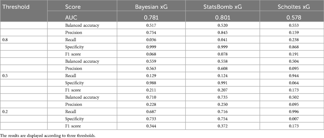
Table 2. Model performance of the Bayesian model, StatsBomb xG, and Scholtes’ model.

Having obtained a reasonable model, we will now illustrate the advantages of the proposed approach and focus on a given international football competition: the FIFA World Cup 2022. First, to underline the impact of the prior used for the Bayesian xG model compared to the prior proposed by Scholtes, we calculated the WIM. This measure is used to compare two distributions, and in the Bayesian framework, to compare two posterior distributions obtained with distinct priors. As suggested in the original paper, we computed the WIM using the uniform prior. The aim of the approach is to evaluate the quantity of information provided by the prior: the higher the WIM between a given prior and the uniform prior, the more informative the prior is. The WIM was computed using the samples obtained with the MCMC algorithm, and resulted in a WIM almost four times higher for the Bayesian xG prior against the uniform prior than for the Scholtes prior against the uniform prior (Table 3).

Table 3

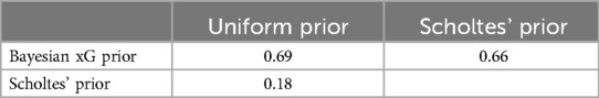
Table 3. Wasserstein Impact Measure using the priors proposed for the Bayesian model and Scholtes’ model and using a uniform prior for all parameters.

To focus on the Bayesian xG model, the maximum a posteriori parameter estimation showed that the distance feature (i.e., the distance between the shot location and the center of the goal) had the greatest negative influence on the predicted xG (see Table 4). Furthermore, the optimal model structure retained for xG prediction includes a random intercept ${\omega }_{\alpha }$ and two random slopes (on angle and closest_opponent parameters, denoted by ${\omega }_{{\beta }_5}$ and ${\omega }_{{\beta }_7}$, respectively). Since ${\omega }_{{\beta }_5}$ and ${\omega }_{{\beta }_7}$ differ from 0, they highlight team-specific traits and relationships between these predictors and the predicted xG. Accordingly, such a model structure allows for consideration of inter-team variability. The univariate posterior and prior distribution for the fixed effects showed the differences between the Bayesian model calibrated on the 2022 FIFA World Cup and the global model fitted on other competitions (see Figure 3). For this competition, the features nb_opponent_on_traj, angle, and body_part_head had a particularly higher negative impact than the global model. This means that in this competition and situation, the players were less likely to score than usual. However, the optimal model retained a random slope on the angle feature, meaning that some teams were significantly better than others to deal with the bad angles.

Table 4

Table 4. Maximum a posteriori parameter estimation for the FIFA World Cup 2022.

Figure 3

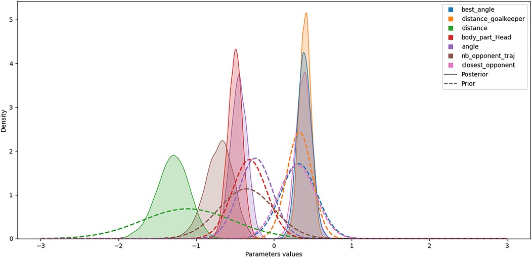
Figure 3. Univariate posterior and prior distribution of the $\mathit{\beta }$ parameters for the 2022 FIFA World Cup.

Computing SHAP values allowed us to explain the model predictions and, for a given shot, to interpret the impact of each feature’s value on the prediction. In addition, we can examine poorly predicted shots to understand where the failure arises from. For example, Figure 4 presents two poorly predicted shots and their respective feature contributions. The first shot has a very high xG value because it is close, central, and there is no opponent on its trajectory. However, the pressure exerted by the nearest opponent likely exceeded the model’s prediction, resulting in a missed shot. The second shot was challenging, characterized by its considerable distance and lateral displacement, with two opposing players present on its trajectory. Nevertheless, the player successfully converted his attempt into a goal.

Figure 4

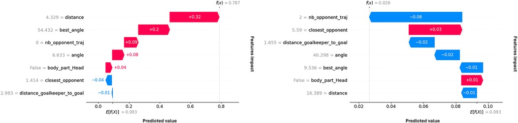
Figure 4. SHAP waterfall plots for two separate shots. The shot on the left has a high Bayesian xG prediction (0.787) and was missed, the one on the right has a low Bayesian xG prediction (0.026) and was scored.

4 Discussion

The present xG mixed-effect model, based on a dataset from the 2022 FIFA World Cup, provided an opportunity to study teams’ goal scoring through strengths and weaknesses in an interpretable and explainable way. The results are arguably of major interest to coaching practitioners, sports scientists, and researchers interested in determining the influence of player and team actions on scoring goals and match outcomes. For practical usage, the models were implemented in a Streamlit web application (33).

Using transfer learning, our model further advances the recent work of Scholtes and Karakuş (21). It can notably undergo an initial pre-training phase on a more extensive and historical dataset and a secondary training phase on a smaller, recent dataset to refine its predictive capabilities. The application of transfer learning within a Bayesian framework yielded results that were comparable to those of a commercial xG model (developed by StatsBomb), despite the utilization of a reduced dataset (see Table 2 for a summary). Furthermore, the interpretability of our linear model is a notable advantage as each model parameter can be analyzed and compared with one another. For instance, the distance from the goal had the most significant influence on xG predictions (over the shot angle) and should, consequently, be considered in any training drills and in-game tactical decision-making.

The Bayesian framework has several advantages. Building an efficient predictive model in a frequentist way implies training a model over a large enough dataset (34). In their study, Robberechts and Davis (35) concluded that five seasons of data were needed to fit an accurate frequentist and non-parametric xG model. Since the Bayesian inference comes with prior distributions, fewer training observations are needed to fit a model correctly. In addition, our approach also addressed confidentiality issues. Identifying a prior distribution implies learning a first function that approximates xG using a separated data sample (in our case, to use another competition to build the baseline model). Through transfer learning, models trained on multiple competitions can be reused for the targeted competition, reducing the computation time and improving model performances. Furthermore, retraining the baseline model on the competition of interest helps identify differences and similarities between the competitions.

In this work, we focused on open-play phases only, while overall, football performance should be modeled from all playing phases. However, the method is transferable to any playing phases where models could be built separately or combined. As aforementioned, player characteristics have significant importance in any football performance modeling. Player-specific data might improve model accuracy and outperform other commercial xG models. Gender has also shown some importance, as mentioned by Bransen and Davis (12). Considering gender in xG modeling or building gender or youth-specific models is recommended. Since football data on the women’s game are generally less abundant, the proposed approach based on transfer learning should address this issue as an optimal model would be built for a given competition while benefiting from broader information.

Even though sports performance modeling remains challenging due to its inherent complexity, analyzing players’ and teams’ characteristics provides essential information for this task. In this study, we considered individuals as teams since the data did not allow us to consider each player individually. Hence, the cross-random effects from the mixed logistic regression highlighted singularities between football teams, particularly regarding the body_part_head and nb_opponent_traj features. However, one may note that player-level information could significantly increase the performance of xG predictions, as players have strengths and weaknesses of their own. Beyond this, the model could allow for adapting a pre-game team strategy or making on-field decisions, to optimize the efficiency of the team.

Expert knowledge can be included in the model as priors. Nevertheless, if the number of observations is insufficient to construct the prior or if the prior information reflects extreme parameter values, there is a risk of bias and identification failure of posterior distributions (36–38). This phenomenon can be observed in our dataset when a comparison is made between the results of Scholtes’ model and the Bayesian xG model that we propose. Indeed, fitting the model by competition results in a smaller dataset than that employed in the aforementioned work. Furthermore, the selection of priors has led to a model with a higher xG prediction than that of StatsBomb and our own model. Conversely, when a sufficient number of observations have been accumulated, the incorporation of expert knowledge as a prior enables coaches to exert direct influence on predictions and decisions, thereby facilitating the provision of valuable real-time feedback. To illustrate, a coach’s knowledge of the game could be incorporated into the prior to facilitate meaningful insight into the players. Knowledge of the strengths of the starting team he has chosen, or of the opposing team, could lead to a manual shift in the value of the parameters influenced. Coaches could then readily utilize the model’s parameters to optimize in-game strategies, such as identifying the optimal shooting distance for individual players and offering practical insights for enhancing overall team performance.

The proposed method may also be of particular interest for modeling expected goals on target (xGOT). xGOT is a post-shot metric that uses the position at which the ball enters the goal and whether it is saved or scored. The xGOT is primarily employed to assess a team’s finishing proficiency by comparing xG with xGOT and to evaluate the performance of goalkeepers according to the quality of the shot. The methodology delineated in this paper also permits the identification of scenarios wherein specific teams exhibit superior finishing proficiency or more efficacious goalkeeping and the characterization of these scenarios. However, although our approach is generalizable to many cases, it is possible that predictive quality may be reduced in tasks that are too complex, such as expected threat. Maintaining high interpretability and, therefore, simple models for such tasks would potentially lead to a greater loss of predictive quality.

5 Conclusion

The development of interpretable and, more widely, explainable artificial intelligence represents a pivotal area of research within the field of computer science and subsequently sports science. This approach facilitates the extraction of novel insights from complex sports data, thereby empowering practitioners to make well-informed decisions (39). Our approach, based on a Bayesian mixed logistic regression model, is aligned with the principles of reproducibility and interpretability. Furthermore, it achieves comparable predictive performance to that of more complex models, despite the utilization of a limited sample of competition data. It also addresses practical concerns such as the identification of team strengths and weaknesses, and could be further extended to model xG from individual characteristics in a straightforward, accessible, and reliable manner.

Data availability statement

The original contributions presented in the study are included in the article/Supplementary Material, further inquiries can be directed to the corresponding author.

Author contributions

LI: Conceptualization, Formal analysis, Investigation, Methodology, Visualization, Writing – original draft, Writing – review & editing, Data curation. SC: Formal analysis, Methodology, Writing – original draft, Writing – review & editing. MR: Data curation, Resources, Writing – original draft, Writing – review & editing. TH: Data curation, Writing – original draft, Writing – review & editing. CC: Writing – original draft, Writing – review & editing, Formal analysis. FI: Conceptualization, Formal analysis, Funding acquisition, Investigation, Methodology, Project administration, Resources, Software, Supervision, Validation, Visualization, Writing – original draft, Writing – review & editing.

Funding

The author(s) declare that no financial support was received for the research and/or publication of this article.

Conflict of interest

The authors declare that the research was conducted in the absence of any commercial or financial relationships that could be construed as a potential conflict of interest.

Generative AI statement

The author(s) declare that no Generative AI was used in the creation of this manuscript.

Publisher's note

All claims expressed in this article are solely those of the authors and do not necessarily represent those of their affiliated organizations, or those of the publisher, the editors and the reviewers. Any product that may be evaluated in this article, or claim that may be made by its manufacturer, is not guaranteed or endorsed by the publisher.

References

1. Ali A. Measuring soccer skill performance: a review. Scand J Med Sci Sports. (2011) 21:170–83. doi: 10.1111/j.1600-0838.2010.01256.x

PubMed Abstract | Crossref Full Text | Google Scholar

2. Sarmento H, Clemente FM, Afonso J, Araújo D, Fachada M, Nobre P, et al. Match analysis in team ball sports: an umbrella review of systematic reviews and meta-analyses. Sports Med Open. (2022) 8:66. doi: 10.1186/s40798-022-00454-7

PubMed Abstract | Crossref Full Text | Google Scholar

3. Sarmento H, Marcelino R, Anguera MT, CampaniÇo J, Matos N, LeitÃo JC. Match analysis in football: a systematic review. J Sports Sci. (2014) 32:1831–43. doi: 10.1080/02640414.2014.898852

PubMed Abstract | Crossref Full Text | Google Scholar

4. Shergill AS, Twist C, Highton J. Importance of GNSS data quality assessment with novel control criteria in professional soccer match-play. Int J Perform Anal Sport. (2021) 21:820–30. doi: 10.1080/24748668.2021.1947017

Crossref Full Text | Google Scholar

5. Agethen P, Otto M, Mengel S, Rukzio E. Using marker-less motion capture systems for walk path analysis in paced assembly flow lines. Procedia Cirp. (2016) 54:152–7. doi: 10.1016/j.procir.2016.04.125

Crossref Full Text | Google Scholar

6. Green S. Assessing the performance of premier league goalscorers. OptaPro Blog. (2012).

Google Scholar

7. Brechot M, Flepp R. Dealing with randomness in match outcomes: how to rethink performance evaluation in European club football using expected goals. J Sports Econom. (2020) 21:335–62. doi: 10.1177/1527002519897962

Crossref Full Text | Google Scholar

8. Cardoso FDS, González-Víllora S, Guilherme J, Teoldo I. Young soccer players with higher tactical knowledge display lower cognitive effort. Percept Mot Skills. (2019) 126:499–514. doi: 10.1177/0031512519826437

PubMed Abstract | Crossref Full Text | Google Scholar

9. Kharrat T, McHale IG, Peña JL. Plus–minus player ratings for soccer. Eur J Oper Res. (2020) 283:726–36. doi: 10.1016/j.ejor.2019.11.026

Crossref Full Text | Google Scholar

10. Spearman W. Beyond expected goals. In: Proceedings of the 12th MIT Sloan Sports Analytics Conference. (2018). p. 1–17.

Google Scholar

11. Anzer G, Bauer P. A goal scoring probability model for shots based on synchronized positional and event data in football (Soccer). Front Sports Act Living. (2021) 3:624475. doi: 10.3389/fspor.2021.624475

Crossref Full Text | Google Scholar

12. Bransen L, Davis J. Women’s football analyzed: interpretable expected goals models for women. In: Proceedings of the AI for Sports Analytics (AISA) Workshop at IJCAI. (2021). Vol. 2021.

Google Scholar

13. Decroos T, Davis J. Interpretable prediction of goals in soccer. In: Proceedings of the AAAI-20 Workshop on Artificial Intelligence in Team Sports. (2019).

Google Scholar

14. Eggels H, Van Elk R, Pechenizkiy M. Explaining soccer match outcomes with goal scoring opportunities predictive analytics. In: 3rd Workshop on Machine Learning and Data Mining for Sports Analytics (MLSA 2016). CEUR-WS.org (2016).

Google Scholar

15. Rathke A. An examination of expected goals and shot efficiency in soccer. J Hum Sport Exerc. (2017) 12:514–29. doi: 10.14198/jhse.2017.12.Proc2.05

Crossref Full Text | Google Scholar

16. Umami I, Gautama DH, Hatta HR. Implementing the expected goal (xG) model to predict scores in soccer matches. Int J Inform Inf Syst. (2021) 4:38–54. doi: 10.47738/ijiis.v4i1

Crossref Full Text | Google Scholar

17. Fryer D, Strümke I, Nguyen H. Shapley values for feature selection: the good, the bad, and the axioms. IEEE Access. (2021) 9:144352–60. doi: 10.1109/ACCESS.2021.3119110

Crossref Full Text | Google Scholar

18. Lundberg SM, Lee S-I. A unified approach to interpreting model predictions. Adv Neural Inf Process Syst. (2017) 30. doi: 10.48550/arXiv.1705.07874

Crossref Full Text | Google Scholar

19. Arenas M, Barceló P, Bertossi L, Monet M. On the complexity of Shap-score-based explanations: tractability via knowledge compilation and non-approximability results. J Mach Learn. (2023) 24:1–58.

Google Scholar

20. Huang X, Marques-Silva J. On the failings of Shapley values for explainability. Int J Approx Reason. (2024) 171:109112. doi: 10.1016/j.ijar.2023.109112

Crossref Full Text | Google Scholar

21. Scholtes A, Karakuş O. Bayes-xG: player and position correction on expected goals (xG) using Bayesian hierarchical approach. Front Sports Act Living. (2024) 6:1348983. doi: 10.3389/fspor.2024.1348983

PubMed Abstract | Crossref Full Text | Google Scholar

22. Lee SY. Bayesian nonlinear models for repeated measurement data: an overview, implementation, and applications. Mathematics. (2022) 10:898. doi: 10.3390/math10060898

Crossref Full Text | Google Scholar

23. Ghaderinezhad F, Ley C, Serrien B. The Wasserstein impact measure (WIM): a practical tool for quantifying prior impact in Bayesian statistics. Comput Stat Data Anal. (2022) 174:107352. doi: 10.1016/j.csda.2021.107352

Crossref Full Text | Google Scholar

24. Plakias S, Kokkotis C, Mitrotasios M, Armatas V, Tsatalas T, Giakas G. Identifying key factors for securing a champions league position in French Ligue 1 using explainable machine learning techniques. Appl Sci. (2024) 14(18):8375. doi: 10.3390/app14188375

Crossref Full Text | Google Scholar

25. StatsBomb. Data from: Statsbomb open data (2023). Available online at: https://github.com/statsbomb/open-data.

Google Scholar

26. Cavus M, Biecek P. Explainable expected goal models for performance analysis in football analytics. In: 2022 IEEE 9th International Conference on Data Science and Advanced Analytics (DSAA). IEEE (2022). p. 1–9.

Google Scholar

27. Hewitt JH, Karakuş O. A machine learning approach for player and position adjusted expected goals in football (soccer). arXiv [preprint]. arXiv:2301.13052 (2023).

Google Scholar

28. Van Roy M, Robberechts P, Yang W-C, De Raedt L, Davis J. Leaving goals on the pitch: evaluating decision making in soccer. arXiv [Preprint]. arXiv:2104.03252 (2021).

Google Scholar

29. Vehtari A, Gelman A, Gabry J. Practical Bayesian model evaluation using leave-one-out cross-validation and WAIC. Stat Comput. (2017) 27:1413–32. doi: 10.1007/s11222-016-9696-4

Crossref Full Text | Google Scholar

30. Yates LA, Aandahl Z, Richards SA, Brook BW. Cross validation for model selection: a review with examples from ecology. Ecol Monogr. (2023) 93:e1557. doi: 10.1002/ecm.1557

Crossref Full Text | Google Scholar

31. Hoffman MD, Gelman A. The No-U-turn sampler: adaptively setting path lengths in Hamiltonian Monte Carlo. J Mach Learn Res. (2014) 15:1593–623.

Google Scholar

32. Salvatier J, Wiecki TV, Fonnesbeck C. Probabilistic programming in python using PyMC3. PeerJ Comput Sci. (2016) 2:e55. doi: 10.7717/peerj-cs.55

Crossref Full Text | Google Scholar

33. Imbach F. Data from: Bayesian modelling of expected goals (2024). Available online at: https://github.com/fimbach/xG_stats.

Google Scholar

34. Andreon S, Weaver B. Bayesian vs Simple Methods. Cham: Springer International Publishing (2015). p. 207–28.

Google Scholar

35. Robberechts P, Davis J. How data availability affects the ability to learn good xG models. In: Machine Learning and Data Mining for Sports Analytics: 7th International Workshop, MLSA 2020, Co-located with ECML/PKDD 2020, Ghent, Belgium, September 14–18, 2020, Proceedings 7. Springer (2020). p. 17–27.

Google Scholar

36. Gifford JA, Swaminathan H. Bias and the effect of priors in Bayesian estimation of parameters of item response models. Appl Psychol Meas. (1990) 14:33–43. doi: 10.1177/014662169001400104

Crossref Full Text | Google Scholar

37. Smid SC, Winter SD. Dangers of the defaults: a tutorial on the impact of default priors when using Bayesian SEM with small samples. Front Psychol. (2020) 11:611963. doi: 10.3389/fpsyg.2020.611963

PubMed Abstract | Crossref Full Text | Google Scholar

38. Van der Vaart AW. Asymptotic Statistics. Cambridge University Press (2000). Vol. 3. doi: 10.1017/CBO9780511802256

Crossref Full Text | Google Scholar

39. Brocherie F, Chassard T, Toussaint J-F, Sedeaud A. Comment on: black box prediction methods in sports medicine deserve a red card for reckless practice: a change of tactics is needed to advance athlete care. Sports Med. (2022) 52:2797–8. doi: 10.1007/s40279-022-01736-6

PubMed Abstract | Crossref Full Text | Google Scholar