 Phillip Papastefanou1*
 Christian S. Zang1
 Thomas A. M. Pugh2,3Daijun Liu2,3Thorsten E. E. Grams1Thomas Hickler4,5
 Anja Rammig1
- 1TUM School of Life Sciences Weihenstephan, Technical University of Munich, Freising, Germany
- 2School of Geography, Earth and Environmental Sciences, University of Birmingham, Birmingham, United Kingdom
- 3Birmingham Institute of Forest Research, University of Birmingham, Birmingham, United Kingdom
- 4Senckenberg Biodiversity and Climate Research Centre, Frankfurt, Germany
- 5Department of Physical Geography, Goethe University, Frankfurt, Germany
Vegetation responds to drought through a complex interplay of plant hydraulic mechanisms, posing challenges for model development and parameterization. We present a mathematical model that describes the dynamics of leaf water-potential over time while considering different strategies by which plant species regulate their water-potentials. The model has two parameters: the parameter λ describing the adjustment of the leaf water potential to changes in soil water potential, and the parameter Δψww describing the typical ‘well-watered’ leaf water potentials at non-stressed (near-zero) levels of soil water potential. Our model was tested and calibrated on 110 time-series datasets containing the leaf- and soil water potentials of 66 species under drought and non-drought conditions. Our model successfully reproduces the measured leaf water potentials over time based on three different regulation strategies under drought. We found that three parameter sets derived from the measurement data reproduced the dynamics of 53% of an drought dataset, and 52% of a control dataset [root mean square error (RMSE) < 0.5 MPa)]. We conclude that, instead of quantifying water-potential-regulation of different plant species by complex modeling approaches, a small set of parameters may be sufficient to describe the water potential regulation behavior for large-scale modeling. Thus, our approach paves the way for a parsimonious representation of the full spectrum of plant hydraulic responses to drought in dynamic vegetation models.
Introduction
Droughts are projected to increase in frequency and intensity within the 21st century (e.g., Dai, 2013; IPCC, 2014) and are expected to have severe effects on whole ecosystems, e.g., inducing large-scale tree mortality and vegetation die-off (Anderegg et al., 2012; Rowland et al., 2015; Choat et al., 2018). Quantifying these effects and their impact on ecosystem function requires robust modeling approaches, which capture the key features of how plants respond to drought. This challenge is particularly acute for estimating plant responses to drought using large-scale dynamic vegetation models (DVMs, e.g., Cramer et al., 2001) that would need to account for a variety of different vegetation types with different hydraulic systems and strategies of responding to drought. One way to classify those strategies is using the concept of isohydricity (Jones and Sutherland, 1991; Tardieu and Simonneau, 1998), which assumes that plant water potential is strongly coupled to stomatal behavior. The classical isohydricity concept differentiates between isohydric plants, which limit stomatal conductance as soil water potential decreases, thereby approaching constant leaf water potentials, and anisohydric plants, which keep their stomata open, continuing photosynthesis and transpiration. Recently, it has been shown that these two strategies form a continuum rather than a dichotomy (Klein, 2014). Furthermore, it seems that regulation of leaf water-potential and stomatal control, the two mechanisms that are assumed to be strongly connected in the original definition of isohydricity, are less interdependent than originally thought (Martínez-Vilalta and Garcia-Forner, 2017) and a range of metrics to assess isohydricity have been proposed (Feng et al., 2019). Nonetheless, it is clear that understanding the likely response of ecosystems to drought will require modeling approaches that explicitly consider the range of possible hydraulic strategies plants can adopt.
Existing hydraulic model frameworks describe the interplay among the leaf- and soil water potentials, stomatal conductance and transpiration under both well-watered and drought conditions. These models implement detailed hydraulic states, such as leaf water potential, stomatal behavior and xylem conductivity (Jones and Sutherland, 1991; Leuning et al., 1995; Tardieu et al., 2015; Mirfenderesgi et al., 2016; Sperry et al., 2016, 2017; Venturas et al., 2018). Many hydraulic models are based on optimization principles to predict stomatal conductance based on hydraulic properties (Mencuccini et al., 2019), but differ in their optimization criteria and conditions. For example, Dewar et al. (2018) maximized carbon gain, whereas Mackay et al. (2015); Sperry et al. (2017), and Venturas et al. (2018) maximized the difference between carbon gains and hydraulic risk. Other approaches control the stimulus responses on physiological or molecular scales (Tardieu et al., 2015). Parameterization of these models beyond the site-scale remains, however, a challenge. For example, Sperry et al. (2016) need to cover a large space of parameter values in their model to account for the observed heterogeneity in hydraulic behaviors. Additionally, the hydraulic model frameworks described above are mostly stand-alone models and often ignore the coupling to other ecosystem processes, which would be necessary for the implementation of ecosystem responses to drought in DVMs.
Dynamic vegetation models have been developed to simulate the impacts of climate change on ecosystem processes, such as photosynthesis, carbon uptake and allocation, growth, competition and mortality, and the interplay between carbon-, water- and (more recently) nutrient cycles, at large scales (Cramer et al., 2001; Smith et al., 2014; Achat et al., 2016). These models usually describe the plant hydraulics by very simple formulations, and only a few have implemented a more detailed hydraulic representation (e.g., Hickler et al., 2006; Xu et al., 2016; Eller et al., 2018; Kennedy et al., 2019). Capturing variation in strategies for leaf water potential regulation has, however, remained a challenge for two reasons: (1) existing hydraulic models are parameterized for specific sites for a given range of environmental drivers, but dynamic vegetation models need to represent a larger scale across which the environmental drivers often differ widely and (2) the parameters of hydraulic models, which define different plant strategies, are not available for a wide range of species or plant functional types needed for large-scale simulations. A high amount of poorly constrained parameters would induce substantial uncertainty in simulations. Thus, the challenge for large-scale modeling is to develop a parsimonious representation of hydraulic behavior (e.g., leaf water potential dynamics), which can capture a range of different strategies of responding to drought, with parameterization still being feasible.
The aims of our study are thus (1) to provide an empirical hydraulic framework that explicitly captures the regulation mechanisms of water potential in different plant species over time, (2) to reproduce observed leaf water potential dynamics, and (3) to provide a generalized set of parameters that reproduces the dynamics across datasets and species. We present a new framework, based on differential equations, which dynamically describes water-potential regulation mechanisms in plants and can be used for implementation in large-scale dynamic vegetation models. It builds on a static isohydricity classification framework developed by Martínez-Vilalta et al. (2014) but goes beyond their approach by considering leaf water potential regulation dynamically over time. We provide parameter estimates for different hydraulic strategies for the parameterization of plant functional types, as commonly used in dynamic vegetation models.
Materials and Methods
Model Description
Principles of Plant Water Flow
Water flows from the roots through the stem to the leaves, where it is released to the atmosphere. Based on these general principles, our model assumes that the water flow is driven by a forcing pressure Δψ(t) that changes over time:
where, Δψs(t) and ψL(t) are the changes in soil and leaf water potential over time, respectively. The gravitational pull is given by ρ⋅g⋅h, where ρ is the sapwood density, g is the gravitational acceleration and h is the canopy height (Table 2). Equation 1 assumes no contributions from plant water storage to Δψ(t).
Modeling the Forcing Potential Under Well-Watered Conditions and Isohydricity
In the absence of water stress, a plant experiences a daily average forcing pressure Δψ, which we here denote as the forcing potential under well-watered conditions Δψww:
where T = 24 h.
Physiologically, the calculation of Δψww is motivated by the isohydrodynamic behavior of plants, which ensures a nearly constant Δψ over time (Domec and Johnson, 2012). Similarly, Martínez-Vilalta et al. (2014) introduced the so-called ‘pull parameter’Λ, which accounts for the pulling capacity of the plant under high (near-zero) soil water potential. In this situation, abundant water is available in the soil. Our approach implicitly assumes that leaf water potential, and thus, stomatal opening (Supplementary Methods S1), responds to changes in soil water potential, either via hydraulic or chemical signals (Larcher, 2003; Kuromori et al., 2018; Yoshida and Fernie, 2018) or by directly affecting the leaf water potential ψL. In the following, we formalize three special cases of isohydricity (Roman et al., 2015), and present a general solution encompassing also the full continuum in between the cases.
Case 1: Extreme isohydric behavior (Figure 1)
Leaf water potential ψL in this case is assumed to be constant (Franco, 1998), thus, the change of ψL(t) with respect to and Δψ decreases as the soil dries (Figure 1, blue line). Here we set ψ(t) to its minimal value ψL,min which is actively maintained by the plant: ψL(t)→ψL,min. This tendency of ψL can be expressed as a differential equation with an adjustment rate r that accounts for response lags:
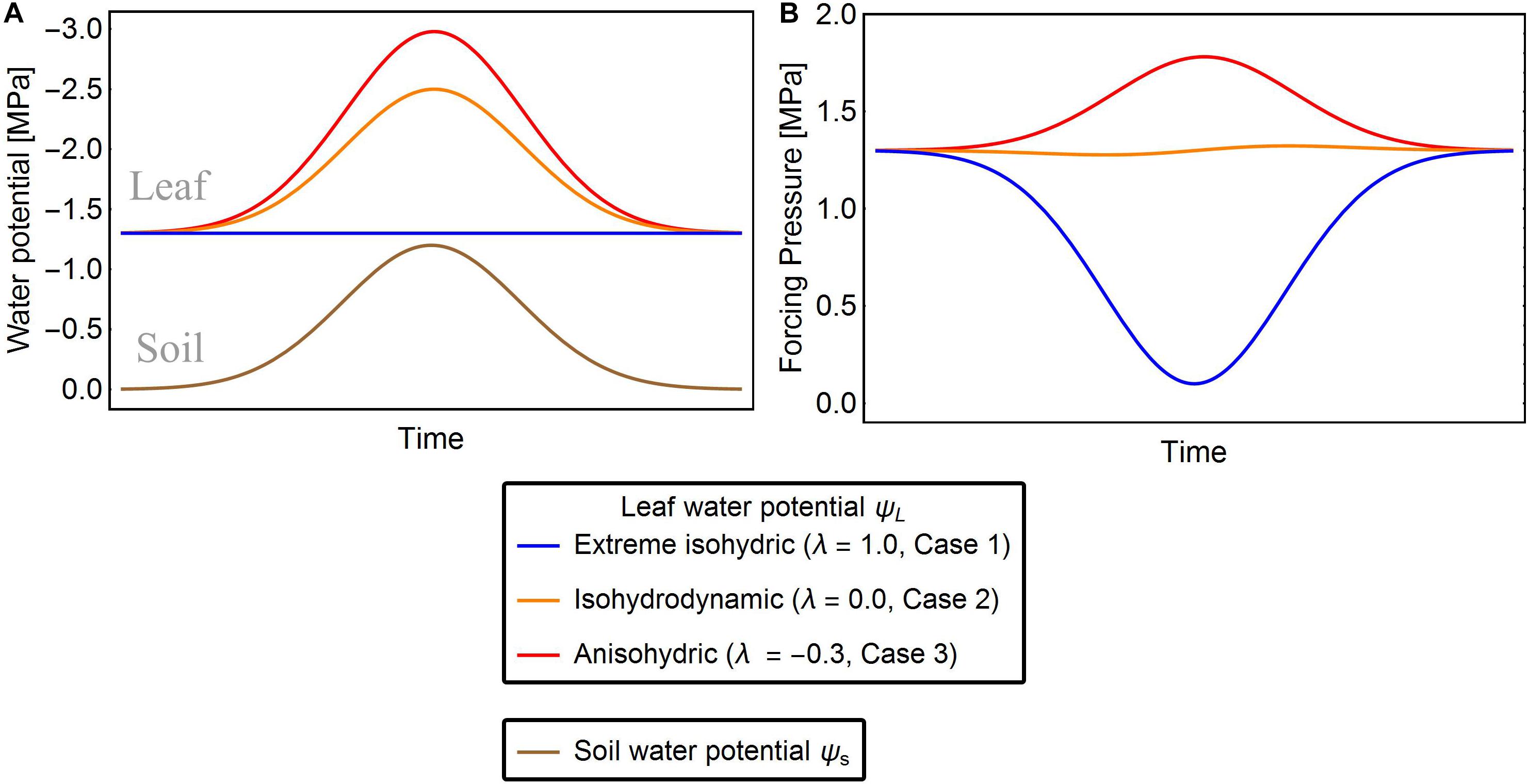
Figure 1. Exemplary solutions of solutions of Eqn. 7 showing ψL (A) and Δψ (B) of the three strategies of water-potential regulation for given ψs. The red, orange, and blue lines are the leaf water potentials for λ = –0.3, 0.0, and 1.0, respectively. In extreme isohydric regulation, a decline in soil water potential does not affect the leaf water potential, but the forcing pressure falls and recovers as the soil water potential drops and rises, respectively (blue lines). In isohydrodynamic regulation, the leaf water potential follows the soil water potential, while the forcing pressure remains constant (orange lines). In anisohydric regulation, the leaf water potential is decreasing and the forcing pressure is increasing with declining soil water potential (red lines).
Assuming that Δψww is reached when the soil water is abundant [i.e., ψs(t) approximates zero], we can relate ψL,min to Δψww as follows:Δψww = ψs(t)−ψL,min≈−ψL,min. The differential equation is then refactored as
Case 2: Isohydrodynamic behavior
In Case 2, plants are assumed to adjust their leaf water potential ψL to follow changes in maintaining a constant forcing pressure Δψ (Figure 1, orange line) and thereby also their maximal stomatal opening. Under constant forcing Δψ→Δψww (Franks et al., 2007), the rate of change in ψL is defined as
The isohydrodynamic behavior described by Eq. (5) adjusts ψL in two ways: (1) If Δψ(t) is lower than the maximum Δψww, it increases until it reaches Δψww; (2) If Δψ(t) is greater than Δψww, it decreases towards Δψww.
Case 3: Anisohydric behavior
Under drought stress, anisohydric plants may adjust their ψL until Δψ increases , hence plants exhibiting anisohydric behavior can potentially adapt their leaf water potentials so that Δψ exceeds Δψww (Figure 1, red line) (Roman et al., 2015). To model this situation, we assume that the leaf water potential tends to M:=q⋅Δψww with q > 1, and refactor Eq. 5 as
Finally, we present a general solution for all three cases, introducing an isohydricity factor λ that captures the transition between the three cases:
Here, λ measures the isohydricity or hydraulic behavior of the water potential regulation. When λ = 1, Eq. (7) reduces to Eq. (4) describing case 1, when λ = 0 it becomes Eq. (5) describing case 2, and when λ < 0 (case 3) we can define by Eq. (7). Assuming that leaf water potential adjusts rapidly on the daily time scale of our study, we set . Note that our modeling approach based on Eq. (7) can simulate the full spectrum of different hydraulic behaviors, including the three special cases described above. Similar frameworks were proposed by Martínez-Vilalta et al. (2014), whose σ measure is inversely related to λ, and by Sperry et al., 2016, who distinguished between isohydricity and anisohydricity by their Slope parameter (which also inversely scales with our λ). However, in contrast to the approach of Martínez-Vilalta et al. (2014), which is static, our model is able to reproduce the dynamics (temporal changes) of ψL across different ψs conditions. Sperry et al., 2016 also capture temporal, diurnal changes in leaf water potential, but require considerably more parameters. Recent studies point toward a non-linear relation between ψL and ψs (Meinzer et al., 2016), which is also considered in our approach, when using small parameter r (i.e., on a sub-daily time scale).
Observational Data
We synthesized publications listed in Martínez-Vilalta et al. (2014) including the measured predawn water potentials (ψPD), the midday water potentials (ψMD) and plant height h (for calculating the gravitational pull) for woody plants. We extracted time series of ψPD and ψMD from each of the publications (Supplementary Data Sheet S1) using WebPlotDigitizer (Rohatgi, 2018). We selected only those datasets containing at least four measurements of ψPD and ψMD over a timespan of at least 2 weeks. Because very few experiments reported the sub-daily measurements of ψL across multiple days, such data were omitted from our analysis. Additionally, we included the dataset from Roman et al. (2015), which already contained the time series of measured ψPD and ψMD in electronic format.
We used ψPD and ψMD as proxies of ψs and ψL, respectively. These assumptions hold if ψs equilibrates overnight with the wettest soil layers around the active roots (Martínez-Vilalta et al., 2014). Under severe drought conditions, overnight equilibration can be insufficient and ψs can exceed ψPD (Xu et al., 2016). The opposite situation (ψs < ψPD) is also possible because root xylem embolism and root shrinkage can create air spaces around the roots, thereby preventing equilibration (Cuneo et al., 2016). These extreme cases, which will violate our proxy assumptions, are excluded from the general parameterization of our model.
In total, we derived 110 time series of 66 species across temperate, tropical, Mediterranean and desert biomes. To sub-divide our dataset, we distinguished between non-drought (‘control’) and drought conditions. Those time series exhibiting pronounced changes in ψPD (varying by at least 1 MPa across the measuring period) were assigned to drought periods. After this division, we derived 66 time series of 48 species for the drought dataset and 44 time series of 44 species for the control dataset. Fourteen species were represented in both, drought and control datasets. The measurements under drought conditions consisted of broadleaved (n = 28) and coniferous tree species (n = 8), shrubs (n = 31). The control measurements consisted mainly of broadleaved (n = 41) and coniferous tree species (n = 9), but also included shrubs (n = 4) (Figure 2A). The data collected under drought conditions were mainly (∼90%) collected from temperate zones (n = 20) and the Mediterranean (n = 42), while only few data were available from deserts (n = 6) and tropical areas (n = 2) (Figure 2B).
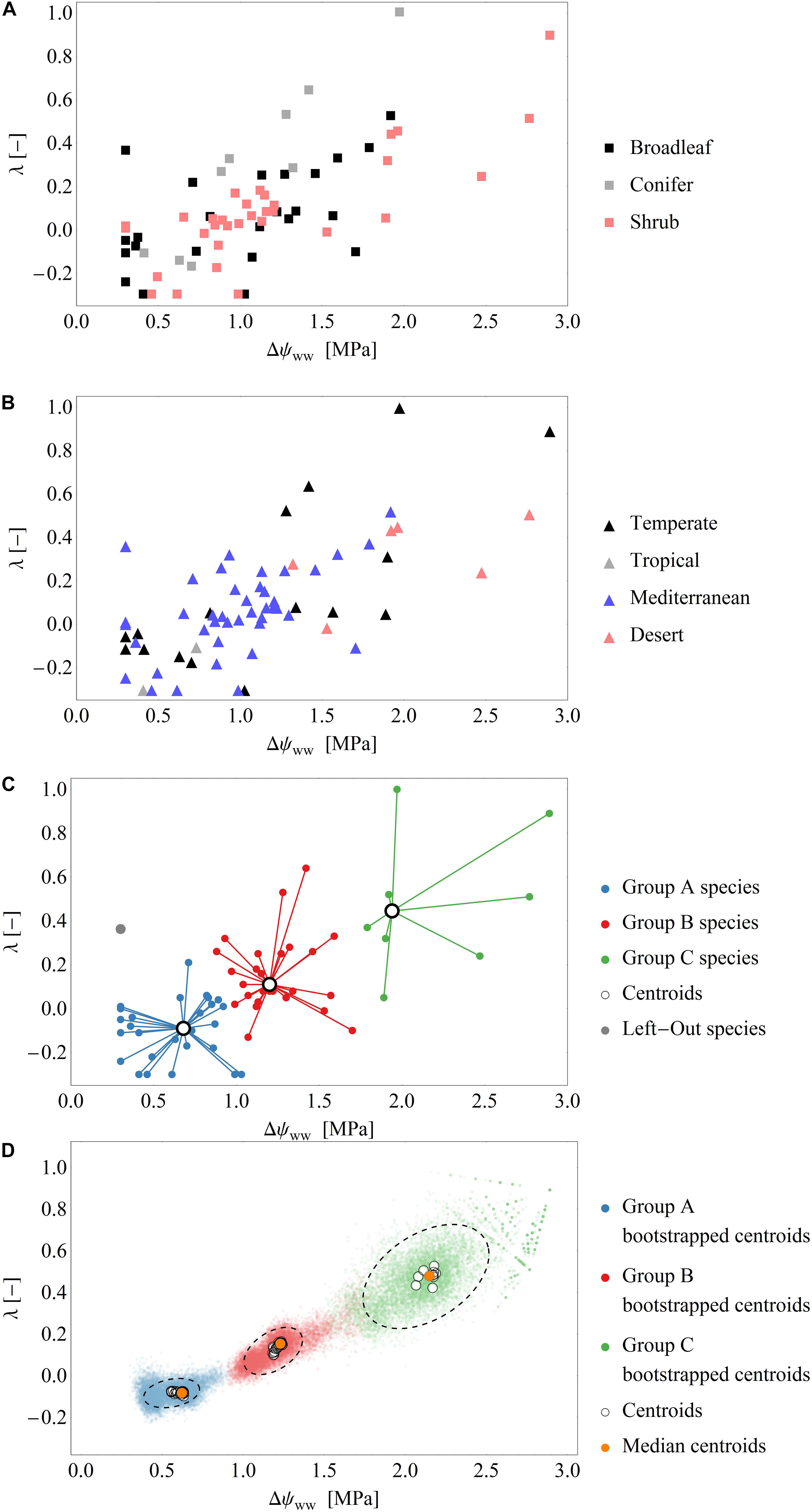
Figure 2. (A,B) Scatterplots of the fitted parameter pairs across the drought dataset, grouped by functional types (A) and biomes (B). (C) Exemplary classification of fitted parameters into the three groups by the cluster analysis using the leave-one-out approach (see also Supplementary Figure S1). Of the 66 data points in the drought dataset 65 points (blue, red, green) are used for clustering and one point (gray) is used for model evaluation. Black open circles are the cluster centroids of the three groups. (D) Results over all clustering analysis performed by the leave-one-out analysis: Blue, green, red dots: Centroids of an additional bootstrapped clustering analysis performed. Black, dashed ellipsis: 90%-quantile-ellipses encompassing 90% of the bootstrapped centroids. Black open circles are the cluster centroids of the three groups of the 66 clustering analysis. Orange dots: Median centroids based on the centroids of each cluster analysis (open circles).
Model Calibration: Estimation of the Parameter Pairs Δψww and λ
The model parameters were calibrated by fitting Eq. (7) to the drought dataset. Using the measured ψPD time series as ψs in Eq. (7), we optimized the parameter pair (Δψww, λ) by minimizing the root mean square error (RMSE) between the observed ψL (measured ψMD) and predicted ψL. We also investigated the stability of the parameter sets by computing a relative root mean square error with being the parameter pair where is a global minimum across the parameter space. To ensure convergence toward a global minimum parameter set, we employed three different heuristic numerical optimization techniques (‘random search,’ ‘simulated annealing’ and ‘differential evolution’; see Supplementary Methods S2). The numerical optimization routines were restricted to certain ranges of λ and Δψww. In particular, λ was limited to λ < 1.0 (Case 1, perfect isohydric behavior) and to at least λ > −0.3 (Case 3, anisohydricity) to scale linearly with cases 1 and 2. Δψww was maintained above 0.3 MPa to allow a minimal positive forcing difference between the leaf- and soil water potentials, which was visible in all of our datasets. These settings are rationalized in the ‘stability analysis’ section below.
Clustering/Grouping of Parameter Pairs and Model Evaluation
We classified the observations in terms of water-potential regulation mechanisms based on a k-means clustering analysis (Python-Package: sklearn) of the model parameters (Δψww, λ). Because of the small size of our dataset we selected the leave-one-out cross validation technique (Efron, 1982) to test the robustness of our approach. Thereby, all points except one from our drought dataset are used to identify three clustering groups and one (left out) point is used for model evaluation. The k-means cluster analysis was also used to predict the corresponding group of the left out point and centroids of the three clusters. This clustering analysis was iterated over all points of the drought dataset resulting in 66 different clustering analyses with three groups, three centroids and one left out point, each.
We calculated the median centroids for each of the three groups over all the clustering analyses. Each median centroid is again a parameter pair (Δψww,λ).
Each left out point was associated with one of the three clustering groups using the k-means cluster analysis. By applying the groups centroid parameter pair, we compared ψL,pred(t) against the time series ψL,obs(t) of the left out data point. As the control dataset was not used for model calibration and hence no group was associated with it, we applied the three median centroids to each point of the control dataset.
The overall prediction skill was evaluated by calculating the RMSE of the observed versus the modeled leaf water potential. Additionally, we evaluated the dynamic behavior of the model, and compared the mean and peak (minimum) leaf water potentials of each of the three groups centroid and the corresponding left out point (Figure 3). Determining the peak leaf water potential under drought stress is reasonable, because the risk of stem (or branch) cavitation is thought to be highest at this potential. Equation (7) was then solved (1) using the associated group’s centroid Δψww and λ values for the drought dataset and (2) using the median centroids of the groups for the control dataset. Next, the time point tP_ obs of the observed peak ψL was identified in each time series, and compared with the predicted peak ψL at tP_ sim. In a given time series, the means and peak values of all observed ψL values were compared against the predicted mean and peak ψL values. The evaluation measure was the RRMSE (Figures 4, 5).
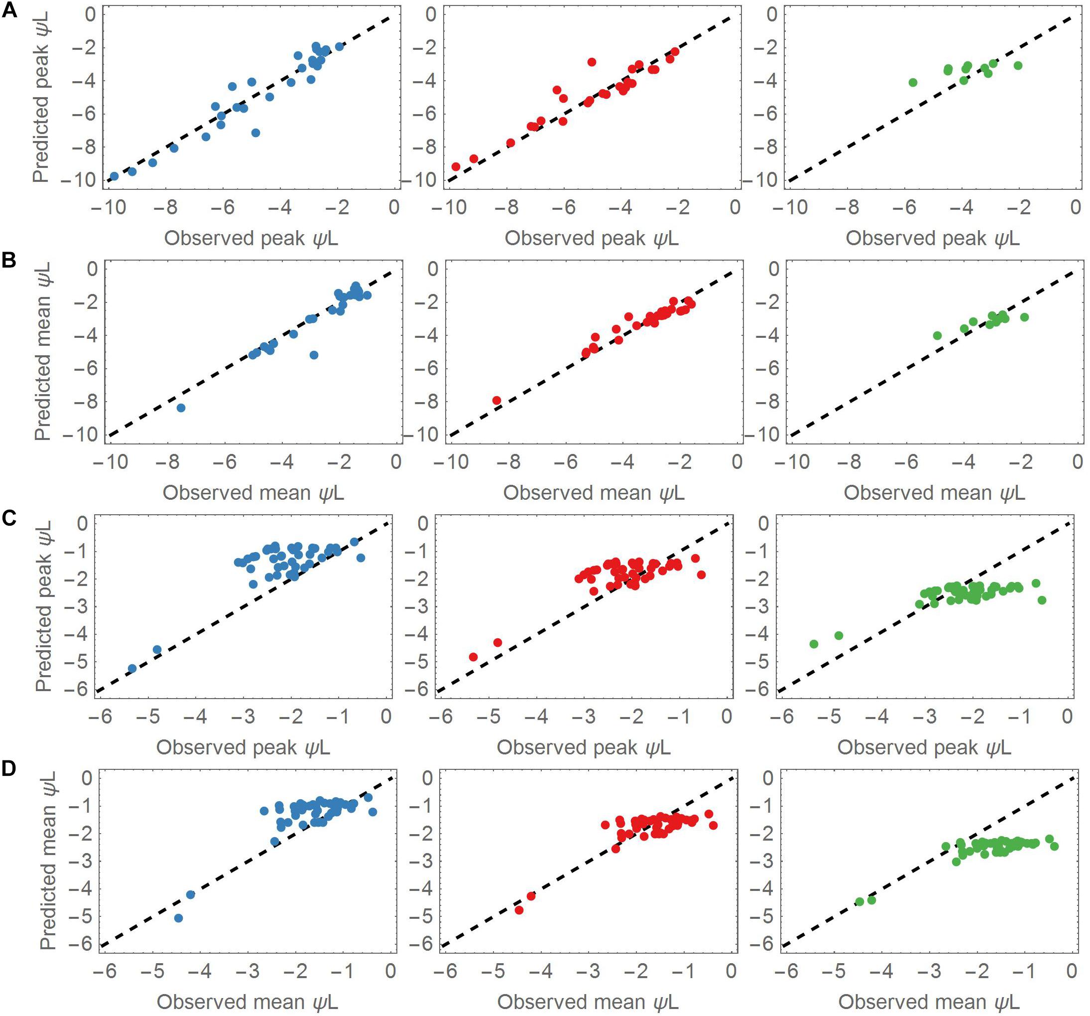
Figure 3. (A) Predicted versus observed peak leaf water potentials in the drought dataset for the three cluster groups. Most of the species are covered by the groups A (Blue points, left column) and B (Red points, middle column). A lower number of species was associated with group C (Green points, right column). (B) As for panel (A), but plotting the mean values of the predicted and observed leaf water potentials. (C) Predicted versus observed peak leaf water potentials applied to all control datasets. The observed peaks aggregate around –2 MPa. (D) As for panel (C), but applying the mean values of the predicted and observed leaf water potentials to the control datasets. The observed means also aggregate around –2 MPa.
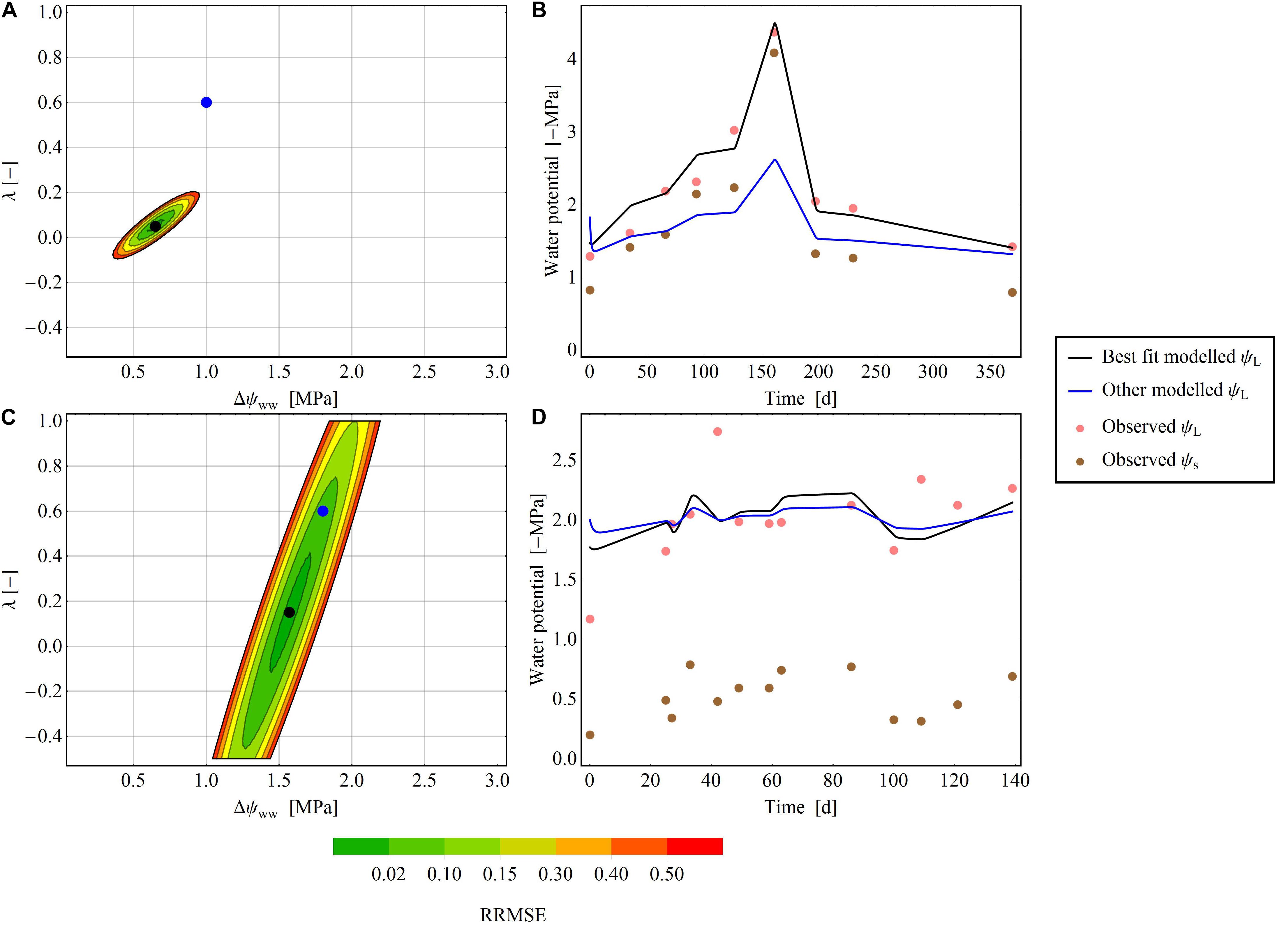
Figure 4. Areas of RMSE deviation from the optimal parameter pair (Δψww and λ) for two exemplary species at two exemplary sites. (A,B) Pratt et al. (2008) dataset, where an exact parameter pair is readily determined. (C,D) Ellsworth and Reich (1992) dataset: an exact determination of the parameter pair is not possible. (A,C) The color gradient shows the RRMSE [from 0 (green) to 0.2 (red)] between the selected and minimal RMSEs. In the white areas of the plot, the RRMSE exceeds 0.2. The black dot denotes the optimal parameter pair in the dataset, and the blue dot is another parameter pair that diverges from the best pair. (B,D) Show the time-series of the modelled ψL for the best fit (black line) and the other fit (blue line) next to observed ψL (pink points) and observed ψs (brown points).
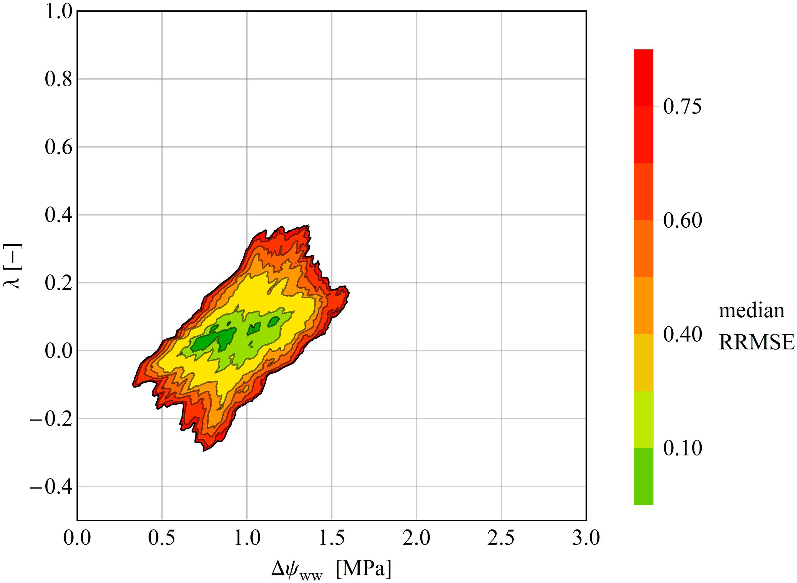
Figure 5. Median RRMSEs at each pixel in the (Δψwwww–, λ) parameter plane, computed over all species of the drought dataset. All values above 3.0 MPa were excluded. Like the clustering analysis, the isohydrodynamic water-potential regulation (Case 2) minimizes the error across the drought datasets. The Δψmax– and λ-axes are each subdivided into 1000 parameter values, giving (1000 × 1000) = 1000.000 pixels in the parameter plane.
Results
Estimated Parameter Pairs
After fitting the model (i.e., Eq. 7) to the drought dataset, we obtained a broad range of both parameters Δψww and λ (mean Δψww = 1.1 MPa, SD = 0.59 MPa; range of Δψww 0.3 to 2.89 MPa and mean λ = 0.1, SD = 0.27; range of λ−0.3 to 1.0, Figures 2A–C). Generally, ∼90% of the time series were best fitted when λ < 0.5, and 33% were best fitted when λ < 0.0. These results indicate a tendency toward isohydrodynamic (Case 2) or anisohydric (Case 3) water-potential regulation of the examined species (Figures 1, 2). In the Δψww fitting, 78 and 27% of the estimated values were lower than 1.5 and 0.75 MPa, respectively.
After grouping the parameter pairs by biomes and functional types, there were no obvious clusters of specific water-potential regulation groups (Figure 2B). The mean λ was 0.06 (SD = 0.19) for the Mediterranean species, 0.17 (SD = 0.39) for the temperate species, and 0.32 (SD = 0.19) for the desert species. The mean Δψww was high for the desert species (2.0 MPa) and lower for the temperate and Mediterranean species (1.18 MPa and 0.97 MPa, respectively). This suggests that (relative to the ψs) the ψL is lower in desert species than in species occupying other habitats. There is some evidence that desert species generally maximize photosynthesis rates rather than minimizing transpiration (e.g., Gibson 1998) which could explain the higher Δψww. The mean λ were similar in broadleaved trees and shrubs (λ = 0.08, SD = 0.25), but higher in conifers (λ = 0.29, SD = 0.39), indicating a more isohydric water-potential regulation).
The mean Δψww values were similar across broadleaved trees, shrubs and conifers (1.0, 1.18, and 1.06 MPa, respectively). Generally, grouping the parameters by biome or functional type did not show a clear separation of the two model parameters. This indicates that in our dataset, the different regulation mechanisms of hydraulic water potential were spread across biomes and functional types.
Clustering of Parameter Pairs and Model Calibration
The cluster analysis results in the splitting of the parameter pairs into three distinguished groups (Table 1). About 44% of species in the drought dataset (29/66) were characterized by low Δψww (mean = 0.61 MPa) and λ (mean = −0.08; group A). A second group (group B, 41% of the drought dataset 27/66) displays higher (moderate) values of Δψww (mean = 1.22 MPa) and λ (mean = 0.15). The remaining 15% (10/66) species from group C with high λ and higher Δψww. Below we describe these three groups and their regulation behavior in more detail:
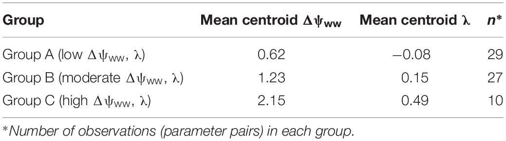
Table 1. Overview of the water-potential regulation groups obtained in the cluster analysis and their mean (Δψww, λ) values.
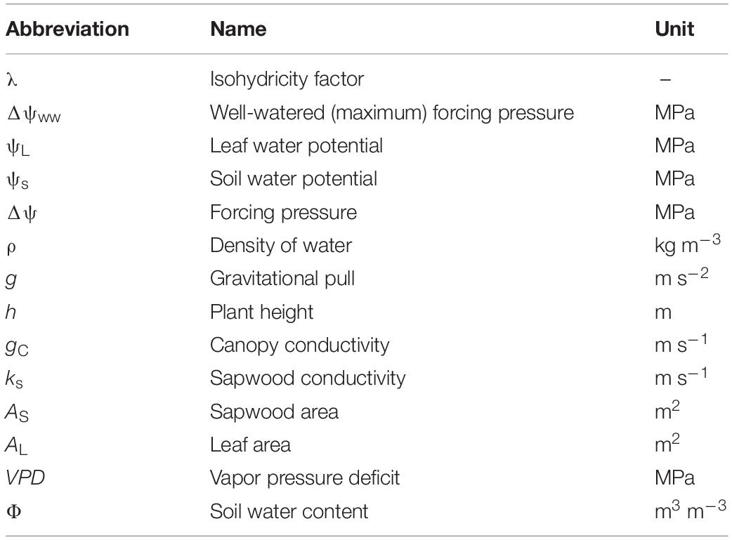
Table 2. Abbreviations, names and units of all variables and parameters used in our modeling approach.
• Group A (low Δψww, λ): Comprising most of the parameter pairs (n = 29), this group was characterized by particularly low values of λ (−0.3 to 0.36, mean = −0.08, SD = 0.16) and low values Δψww (0.3–1.03 MPa, mean = 0.62 MPa, SD = 0.25 MPa). Species in this group lie between isohydrodynamic and anisohydric water-potential regulators (Cases 2 and 3), which strongly adapt their ψL to changes in ψs.
• Group B (moderate Δψww, λ): The second largest group (n = 27) was also characterized by low λ (−0.13 to 0.64, mean = 0.15, SD = 0.17), but higher values of Δψww (0.88 to 1.7 MPa, mean = 1.23 MPa, SD = 0.21 MPa). The water potential regulation in this group settles between isohydric and isohydrodynamic (Cases 1 and 2). Group B species adopt less strongly to changes in the soil water potential compared to species of group A. Because of their higher Δψww values compared to group A, plants of this group generally operate at lower levels of ψL (relative to ψs) than group A species.
• Group C (high Δψww, λ): The smallest group in the clustering analysis (n = 10) was characterized by higher λ values compared to group A and B (mean = 0.48, SD = 0.28) and hence by a more isohydric water-potential regulation. The higher Δψww values in this group (mean = 2.15 MPa, SD = 0.4 MPa) imply also operation at lower levels of ψL (relative to ψs).
About 44% (29 out of 66) entries in the drought dataset were assigned to the low-Δψww, λ group (group A), indicating that a large part of our dataset could be described by an isohydrodynamic water-potential regulation parameterization of our model (Cases 2 and 3). Species in this group strongly adjust their ψL after a drop in ψs. This group also spans a range of low Δψww, indicating that under unstressed conditions, isohydrodynamic water-potential regulation is associated with low gradients. Almost the same amount of entries (27 out of 66) in the drought dataset were assigned to the moderate Δψww group (group B). In contrast to group A entries of group B had slightly higher λ and considerably higher Δψww values. The water-potential regulation of group B species is less anisohydric compared to group A, tending more toward isohydrodynamic behavior. The higher Δψww implies that species of this group generally operate at lower levels of ψL (relative to ψs). A minority of species (10/66) were assigned to the high Δψww group (group C). The high values of Δψww indicate that species associated with this group generally operate at low levels of ψL relative to ψs, however, are less vigorously adjusting ψL to decreases in ψs than the groups A and B. Species of group C can be considered as being between isohydric and isohydrodynamic, but tending more toward isohydric behavior.
Model Evaluation of the Clustered Groups
The parameter sets of group A (low Δψww) and B (moderate Δψww) represented most of the dynamics of the drought dataset. Overall, group A and B adequately predicted the mean and peak leaf water potentials of the drought dataset (Figures 3A,B). The mean RMSE of the predicted leaf water potential in Group A was 0.51 MPa, whereas the observed and predicted peak ψL values in the drought dataset ranged from −1.93 to −9.81 MPa, <reflecting the wide range of ψL covered by this dataset and the prediction. Both the observed and predicted ψL peaks varied largely across the dataset (mean = −4.65 MPa, SD = 2.19 MPa). Similarly, group B accurately explained ψL time series of the 27 points associated with it (mean RMSE = 0.52 MPa). The peak ψL observed and predicted of group B covered a slightly wider range from −2.11 to −12.03 MPa with similar variability but lower peak ψL (mean = −5.56 MPa, SD = 2.65 MPa). With a mean RMSE = 0.63 MPa, group C captured ψL time series of its 10 associated species with less accuracy. Compared to the species of group A and B the species associated with group C had higher observed and predicted ψL ranging from −2.04 to −5.72 MPa. Its values centered around higher values of peak ψL with lower variability (mean = −3.75 MPa, SD = 1.02 MPa).
The mean observed ψL of group A was significantly higher than the peak observed ψL ranging from −1.03 to −7.54 MPa with mean around −2.66 MPa. Again, group B showed a similar range of mean observed ψL from −1.62 MPa to −8.43 MPa and a more negative mean of −3.37 MPa. The differences compared to peak observed ψL reflect the strong changes of ψL in the measuring period, and a tendency toward anisohydric or isohydrodynamic water-potential regulation. Group C showed mean observed ψL ranging from −1.88 to −4.92 MPa which is closer to the peak observed ψL compared to groups A and B. This indicates the more isohydric behavior of species associated with this group as they do not lower their leaf water potential under changing ψL as strong as group A and B.
The observed ψL peaks in the control datasets ranged from −0.54 to −8.92 MPa (mean observed ψL range −0.38 to −7.82 MPa), with both peaks and means clustered around −2 MPa. The smaller difference in mean and peak ψL indicates less pronounced changes of ψL within the measuring period (Figures 3C,D). These findings show that under non-drought conditions, most of the plants stabilized their ψL around −2 MPa. Group A and B best predicted the leaf water potential time series ψL in the control time series (with RMSEs of 0.58 and 0.55 MPa, respectively). Group C performed worse in predicting the ψL time series (RMSE = 1.02 MPa).
Stability Analysis in the 2D Parameter Plane
In some time series, the RRMSE was restricted to a small area of the parameter space, indicating one parameter pair that describers the regulation mechanism of the water potential according to the parameter λ (Figure 4A). This means, that predictions using the best fitting ψL trace time series of observed ψL much more closely than alternative predictions based on different parameter pairs (Figure 4B). For other time series the RRMSEs around the best parameter pair covered a larger area, resulting in ambiguous parameterization of Δψww and λ in the time series (Figure 4C). Here, different pairs of (Δψww, λ) can describe the observed dataset and consequently a single regulation mechanism of water potential cannot be identified (Figure 4D). After averaging the RRMSEs across the drought dataset for each pixel (Δψww, λ) in the parameter plane, the median lowest errors were determined as 0.6 MPa <Δψww<1.4 MPa, and −0.5 < λ < 0.125 (Figure 5), consistent with the median centroids of groups A and B.
Discussion
Strategies of Leaf Water Potential Regulation
We found the majority of species displaying more isohydrodynamic regulation of their leaf water potential (Case 2, Figure 1). In contrast, strong isohydric water potential regulation (Case 1, Figure 1) was found in only a few cases. However, we found a large variability within these hydraulic strategies, which is reflected by the large spread of our model parameter λ across species, in agreement with findings of Martínez-Vilalta et al. (2014).
When reducing the heterogeneity of our model parameter λ to only a small set of parameter pairs (Δψww, λ), we could successfully reproduce the water-potential-regulation dynamics of the considered species under both drought and control conditions. The model showed better performance in predicting the responses to drought compared to the control responses (Figure 3). This may be because our model is particularly designed to only capture drought responses to declining levels of ψs; Under control conditions with constant ψs only other environmental drivers may influence ψL, which are not covered by our approach.
In particular, group A and B in the cluster analysis explained a wide range of the leaf water-potential dynamics (Figure 3) across species. These two groups represent plants that isohydrodynamically regulate their water potential by maintaining a constant forcing potential Δψ (Figure 1). The differences in hydraulic behavior between the two groups A and B mainly arise (according to the clustering) from their operational levels of ψL under drought and control conditions. With a higher Δψww species associated with group B are generally working at lower levels of ψL compared to species of group A. This indicates that species of group B might be slightly more drought resistant than species of group A.
This reduction of parameters is especially relevant for dynamic vegetation modeling, because models often assume extreme isohydric water-potential regulation in plants (e.g., Hickler et al., 2006), which rarely occurred in our dataset. Differences in hydraulic behavior such as water-potential regulation can have substantial implications for ecosystems. For instance, more anisohydric behavior may substantially influence evapotranspiration fluxes. Furthermore, above 85% loss of conductivity induced by cavitation trees experience widespread mortality (Venturas et al., 2018).
Group C comprised less species of our dataset and also its prediction skill was lower, which might be either because, the more isohydric strategies were not widely spread across species, or (more likely) because our dataset was biased toward European and North American species and Mediterranean and temperate biomes (see section Materials and Methods). Additionally, our dataset was biased toward broadleaved species. Thus, the lack of significant differences in the water potential regulations between conifer and broadleaved species may result from the low representation of conifer species. The absolute levels of soil water potentials varied across species and sites, especially in the drought- but also in the control-datasets. Thus, our approach not only captured the differences in hydraulic strategies, but also the intensity in differences between the normal and drought treatments, and the different environmental conditions, which are implicitly reflected in ψs.
Stability of Model Parameters Versus Input Datasets
In the stability analysis, we found large differences in the uniqueness of the model parameter pairs (Δψww, λ) across datasets, environmental conditions and species. Some datasets yielded a clearly determined parameter pair (Δψww, λ) (Figures 4A,B), with a RMSE that rapidly increased with increasing distance from the best fit pair; other datasets yielded a larger set of parameter pairs with equal RMSEs (Figures 4C,D). Generally, the fitting achieved more unequivocal parameter pairs (Δψww, λ), which could be more distinctly attributed to a water-potential regulation strategy from time series with (1) a longer measuring period, (2) a larger number of sample/measuring points, and (3) a larger variety in ψs over time. This indicates that the quality of a unique parameter pair (Δψww, λ), and hence the integrity of the predicted water-potential regulation strategy, depends on capturing both drought and non-drought conditions within the dataset. In control treatments with constant high ψs (close to zero), multiple parameter pairs (Δψww, λ) produced similar ψL, so the regulation mechanism of the water potential cannot be clearly defined (Figure 4D).
Model Limitations
Our model focuses on describing leaf water potential from changes in soil water potential assuming that leaf water-potential regulation can be modeled independently of VPD. However, VPD has a strong influence on hydraulic conductance of plants, in particular during drought, when high VPD leads to decreasing whole-plant hydraulic conductance and increasing canopy temperature (Zhang et al., 2017), indicating stomatal closure of plants to prevent water loss. Stomatal closure reduces transpiration, which is crucial for cooling leaves under high ambient air temperatures often associated with severe droughts (Teskey et al., 2015). Therefore, drought-stressed plants face a trade-off between leaf overheating bearing the risk of potential severe leaf damage, and low xylem-water potential bearing the risk of cavitation. The drought datasets applied here were measured in rainfall exclusion experiments or artificial drought experiments, often only prevent rainwater from reaching the soil (da Costa et al., 2010), but rarely account for impacts of persistent atmospheric dryness under extreme drought (Liu et al., 2015, 2018) and may thus underestimate the impacts of drought. To fully represent the ecosystem responses under drought, such feedbacks need to be considered in drought experiments and implemented in vegetation models. Here, we neglected the direct influence of VPD on the leaf water potential, mainly because time series of VPD were available only for a limited number of datasets. However, when deriving the stomatal conductance from leaf water potential, VPD cannot be excluded as a driving factor (Medlyn et al., 2011).
Another important mechanism that needs to be considered when modeling leaf water potential, is that even when stomata are closed, plants continue to loose water through the stomata and the cuticle (Duursma et al., 2019). In particular, under extreme drought conditions and consecutive days of high VPD, cuticular water loss plays an important role. This water loss reduces the xylem water potential, and may potentially cause plant death by cavitation (Choat et al., 2018). Future hydraulic models should also incorporate water loss through both, leaf cuticula and closed stomata during severe droughts (Duursma et al., 2019).
Our present study focused on the regulation of water potential in plants. Explicit formulations of the water storage capacities of stems, leaves and roots, which are incorporated in other approaches (Xu et al., 2016), were not considered, primarily because of a lack of parameterization data. Although the stem water potential and stem water capacity are correlated, their dynamics and interactions are complex and differ across species. In our model, the parameter r can be interpreted as a storage capacity because changes in r would cause temporal shifts of ψL relative to ψs. Because none of the time series in the datasets showed a visible lag effect of ψL to changes in ψs we set a high value of r = 1 (implying lags of less than 1 day). However, the species and/or regions of the experiments may have been insensitive to capacitance. Where capacitance is known to be important, as in some tropical species (Borchert and Pockman, 2005), this assumption may need to be revisited.
Relating the Leaf Water-Potential Regulation and Canopy Conductivity Implications for Implementations in Dynamic Vegetation Models
We provide a possibility to connect leaf water potential regulation and the forcing pressure Δψ to canopy conductivity (Supplementary Methods S1) based on the principle that the imposed transpiration flux balances the sapwood flux induced by the forcing pressure Δψ (Whitehead et al., 1984). The forcing pressure Δψ and canopy conductivity can be linked by Darcy’s law (McDowell et al., 2016). By this link, the effects of leaf water potential regulation can be used to estimate to canopy conductivity and stomatal behavior according to the three special cases: A decrease of Δψ of extreme isohydric plants (case 1, Figure 1) would lead to a decrease in canopy conductivity gC, reduced transpiration, and consequent reduction in photosynthesis and carbon uptake. Keeping Δψ constant under drying soil requires maintaining a high gC (isohydrodynamic plants, case 2), ensuring that transpiration and photosynthesis continue under increasingly dry conditions. However in this case, xylem cavitation under severe soil-moisture stress can decrease the gC, thus lowering the xylem conductivity ks. Finally, anisohydric plants (case 3) adjust their ψL until Δψ actually increases (Figure 1). Plants adopting this strategy maintain a high gC and high transpiration- and photosynthesis rates, even under strong drought stress. Loss of xylem conductivity ks induced by cavitation is compensated by the decrease in ψL and increase in Δψ. For a summary of the three cases see also Supplementary Methods S3.
Changes in leaf water potential are commonly simulated by differential equations in dynamic vegetation models (Xu et al., 2016; Eller et al., 2018). However, the differences in isohydricity or the regulation mechanisms of water potential are not parametrized in these models. Our new approach explicitly accounts for the differences in water potential mechanisms among plant species by specifying two parameters (Δψww and λ) and can be applied in dynamic vegetation models. Our model is also technically capable of simulating water potential dynamics on sub-daily timescales. However, this is not tested here, because sub-daily measurements of leaf water potential across many consecutive days are expensive and only available from very few experiments.
If the median cluster parameter pairs of our cluster groups A, B, C indeed represents a major fraction of plants, it can be generalized to many vegetation models. However, this tentative conclusion must be tested by further analysis. Furthermore, dynamic vegetation models increasingly aim to capture trait diversity and to understand its implications for ecosystem resilience (e.g., Scheiter et al., 2013; Sakschewski et al., 2016). Here, we could derive the trait gradients encapsulating different regulation strategies of leaf water potentials. Finally, to improve the accuracy of the leaf water-potential dynamics for a specific species, the model parameters can be derived if species-specific time-series of the predawn and midday leaf water potentials would be available (Supplementary Tables S1, S2).
Conclusion
We presented a novel modeling approach that captures the temporal dynamics of regulation strategies of leaf water potentials in plants under changing soil water potentials, with strategies ranging from extreme isohydric (case 1), through isohydrodynamic (case 2), to anisohydric (case 3). With only two parameters (Δψww and λ, assuming r = 1), our model captures different water potential regulation mechanisms across species accurately on a daily scale. Although we did not find a general solution for leaf water potential regulation across all species, many species’ leaf water potential regulation could be modeled using one particular parameter combination. We suggest that when implementing our framework into dynamic vegetation models, a few parameter combinations may be enough to model the leaf water potential regulation across the available plant functional types. To verify this, it is needed to test, in particular, whether the parameter λ can represent (1) a constant parameter, (2) a species-specific trait parameter or (3) a dynamic property of a species. This question arises because parameterizations of our groups A, B and C adequately represented many different datasets, species and environmental conditions.
Our results (especially the successful application of the mean parameter sets of λ and Δψmax) show that the isohydricity concept of water-potential regulation in our and other approaches (e.g., Martínez-Vilalta et al., 2014) cannot explain the hydraulic differences among plant species. Alongside water potential regulation, we should further investigate the different stomatal behaviors and hydraulic safety margins, and the relations among them (Anderegg et al., 2018). Overall, our parsimonious approach offers two main advantages: (1) it is easily tested against observations of leaf- and soil water potentials, and (2) it is easily implemented in dynamic vegetation models to predict leaf-water-potential over time.
Data Availability Statement
The time-series of the dataset analyzed in this manuscript can be found in the Supporting Information. Requests for a complete list of journal articles investigated by this study should be directed to cGFwYXN0ZWZhbm91QGdtYWlsLmNvbQ==.
Author Contributions
PP and AR conceived the study and wrote the first draft of the manuscript. All authors contributed to the development of the model and to the writing of the manuscript.
Funding
PP and AR acknowledge funding from the BMBF- and Belmont Forum-funded project “CLIMAX: Climate services through knowledge co-production: A Euro-South American initiative for strengthening societal adaptation response to extreme events”, FKZ 01LP1610A. CZ acknowledges funding by the Bavarian Ministry of Science and the Arts in the context of the Bavarian Climate Research Network (BayKliF). DL and TP acknowledge support from the European Research Council under the European Union Horizon 2020 programme (Grant 758873, TreeMort).
Conflict of Interest
The authors declare that the research was conducted in the absence of any commercial or financial relationships that could be construed as a potential conflict of interest.
Acknowledgments
We thank Jordi-Martinez Vilalta for valuable comments and sharing a dataset consisting of studies where leaf water potential time-series have been conducted. This is paper number 39 of the Birmingham Institute of Forest Research. Furthermore, we thank Johannes Haas and Sophia Chong for digitizing the time-series data.
Supplementary Material
The Supplementary Material for this article can be found online at: https://www.frontiersin.org/articles/10.3389/fpls.2020.00373/full#supplementary-material
DATASHEET S1 | Time series of predawn and midday leaf water potential.
References
Achat, D. L., Augusto, L., Gallet-Budynek, A., and Loustau, D. (2016). Future challenges in coupled C–N–P cycle models for terrestrial ecosystems under global change: a review. Biogeochemistry 131, 173–202. doi: 10.1007/s10533-016-0274-9
Anderegg, W. R. L., Berry, J. A., Smith, D. D., Sperry, J. S., Anderegg, L. D. L., and Field, C. B. (2012). The roles of hydraulic and carbon stress in a widespread climate-induced forest die-off. Proc. Natl. Acad. Sci. U.S.A. 109, 233–237. doi: 10.1073/pnas.1107891109
Anderegg, W. R. L., Konings, A. G., Trugman, A. T., Yu, K., Bowling, D. R., Gabbitas, R., et al. (2018). Hydraulic diversity of forests regulates ecosystem resilience during drought. Nature 561, 538–541. doi: 10.1038/s41586-018-0539-7
Borchert, R., and Pockman, W. T. (2005). Water storage capacitance and xylem tension in isolated branches of temperate and tropical trees. Tree Physiol. 25, 457–466. doi: 10.1093/treephys/25.4.457
Choat, B., Brodribb, T. J., Brodersen, C. R., Duursma, R. A., López, R., and Medlyn, B. E. (2018). Triggers of tree mortality under drought. Nature 558, 531–539. doi: 10.1038/s41586-018-0240-x
Cramer, W., Bondeau, A., Woodward, F. I., Prentice, I. C., Betts, R. A., Brovkin, V., et al. (2001). Global response of terrestrial ecosystem structure and function to CO2 and climate change: results from six dynamic global vegetation models. Glob. Chang. Biol. 7, 357–373. doi: 10.1046/j.1365-2486.2001.00383.x
Cuneo, I. F., Knipfer, T., Brodersen, C. R., and McElrone, A. J. (2016). Mechanical failure of fine root cortical cells initiates plant hydraulic decline during drought. Plant Physiol. 172, 1669–1678. doi: 10.1104/pp.16.00923
da Costa, A. C. L., Galbraith, D., Almeida, S., Portela, B. T. T., da Costa, M., and de Athaydes Silva, J.Jr. et al. (2010). Effect of 7 yr of experimental drought on vegetation dynamics and biomass storage of an eastern Amazonian rainforest. New Phytol. 187, 579–591. doi: 10.1111/j.1469-8137.2010.03309.x
Dai, A. (2013). Increasing drought under global warming in observations and models. Nat. Clim. Chang. 3, 52–58. doi: 10.1038/nclimate1633
Dewar, R., Mauranen, A., Mäkelä, A., Hölttä, T., Medlyn, B., and Vesala, T. (2018). New insights into the covariation of stomatal, mesophyll and hydraulic conductances from optimization models incorporating nonstomatal limitations to photosynthesis. New Phytol. 217, 571–585. doi: 10.1111/nph.14848
Domec, J. C., and Johnson, D. M. (2012). Does homeostasis or disturbance of homeostasis in minimum leaf water potential explain the isohydric versus anisohydric behavior of Vitis vinifera L. cultivars? Tree Physiol. 32, 245–248. doi: 10.1093/treephys/tps013
Duursma, R. A., Blackman, C. J., Lopéz, R., Martin-StPaul, N. K., Cochard, H., and Medlyn, B. E. (2019). On the minimum leaf conductance: its role in models of plant water use, and ecological and environmental controls. New Phytol. 221, 693–705. doi: 10.1111/nph.15395
Efron, B. (1982). The Jackknife, the Bootstrap and Other Resampling Plans. Philadelphia, PA: Society for Industrial and Applied Mathematics, doi: 10.1137/1.9781611970319
Eller, C. B., Rowland, L., Oliveira, R. S., Bittencourt, P. R. L., Barros, F. V., Da Costa, A. C. L., et al. (2018). Modelling tropical forest responses to drought and El Niño with a stomatal optimization model based on xylem hydraulics. Philos. Trans. R. Soc. B Biol. Sci. 373:20170315. doi: 10.1098/rstb.2017.0315
Ellsworth, D. S., and Reich, P. B. (1992). Water relations and gas exchange of Acer saccharum seedlings in contrasting natural light and water regimes. Tree Physiol. 10, 1–20. doi: 10.1093/treephys/10.1.1
Feng, X., Ackerly, D. D., Dawson, T. E., Manzoni, S., McLaughlin, B., Skelton, R. P., et al. (2019). Beyond isohydricity: the role of environmental variability in determining plant drought responses. Plant. Cell Environ. 42, 1104–1111. doi: 10.1111/pce.13486
Franco, A. C. (1998). Montana, an evergreen savanna species. Plant Ecol. 136, 69–76. doi: 10.1023/A:1009763328808
Franks, P. J., Drake, P. L., and Froend, R. H. (2007). Anisohydric but isohydrodynamic: seasonally constant plant water potential gradient explained by a stomatal control mechanism incorporating variable plant hydraulic conductance. Plant Cell Environ. 30, 19–30. doi: 10.1111/j.1365-3040.2006.01600.x
Hickler, T., Prentice, I. C., Smith, B., Sykes, M. T., and Zaehle, S. (2006). Implementing plant hydraulic architecture within the LPJ dynamic global vegetation model. Glob. Ecol. Biogeogr. 15, 567–577. doi: 10.1111/j.1466-8238.2006.00254.x
IPCC (2014). Climate Change 2013 - The Physical Science Basis. Intergovernmental Panel on Climate Change. Cambridge, UK: Cambridge University Press. doi: 10.1017/CBO9781107415324
Jones, H. G., and Sutherland, R. A. (1991). Stomatal control of xylem embolism. Plant Cell Environ. 14, 607–612. doi: 10.1111/j.1365-3040.1991.tb01532.x
Kennedy, D., Swenson, S., Oleson, K. W., Lawrence, D. M., Fisher, R., Lola da Costa, A. C., et al. (2019). Implementing plant hydraulics in the community land model, version 5. J. Adv. Model. Earth Syst. 11, 485–513. doi: 10.1029/2018MS001500
Klein, T. (2014). The variability of stomatal sensitivity to leaf water potential across tree species indicates a continuum between isohydric and anisohydric behaviours. Funct. Ecol. 28, 1313–1320. doi: 10.1111/1365-2435.12289
Kuromori, T., Seo, M., and Shinozaki, K. (2018). ABA transport and plant water stress responses. Trends Plant Sci. 23, 513–522. doi: 10.1016/j.tplants.2018.04.001
Leuning, R., Kelliher, F. M., de Pury, D. G. G., and Schulze, E. −D. (1995). Leaf nitrogen, photosynthesis, conductance and transpiration: scaling from leaves to canopies. Plant Cell Environ. 18, 1183–1200. doi: 10.1111/j.1365-3040.1995.tb00628.x
Liu, D., Ogaya, R., Barbeta, A., Yang, X., and Peñuelas, J. (2015). Contrasting impacts of continuous moderate drought and episodic severe droughts on the aboveground-biomass increment and litterfall of three coexisting Mediterranean woody species. Glob. Chang. Biol. 21, 4196–4209. doi: 10.1111/gcb.13029
Liu, D., Ogaya, R., Barbeta, A., Yang, X., and Peñuelas, J. (2018). Long-term experimental drought combined with natural extremes accelerate vegetation shift in a Mediterranean holm oak forest. Environ. Exp. Bot. 151, 1–11. doi: 10.1016/j.envexpbot.2018.02.008
Mackay, D. S., Roberts, D. E., Ewers, B. E., Sperry, J. S., McDowell, N. G., and Pockman, W. T. (2015). Interdependence of chronic hydraulic dysfunction and canopy processes can improve integrated models of tree response to drought. Water Resour. Res. 51, 6156–6176. doi: 10.1002/2015WR017244
Martínez-Vilalta, J., and Garcia-Forner, N. (2017). Water potential regulation, stomatal behaviour and hydraulic transport under drought: deconstructing the iso/anisohydric concept. Plant Cell Environ. 40, 962–976. doi: 10.1111/pce.12846
Martínez-Vilalta, J., Poyatos, R., Aguadé, D., Retana, J., and Mencuccini, M. (2014). A new look at water transport regulation in plants. New Phytol. 204, 105–115. doi: 10.1111/nph.12912
McDowell, N. G., Williams, A. P., Xu, C., Pockman, W. T., Dickman, L. T., Sevanto, S., et al. (2016). Multi-scale predictions of massive conifer mortality due to chronic temperature rise. Nat. Clim. Chang. 6, 295–300. doi: 10.1038/nclimate2873
Medlyn, B. E., Duursma, R. A., Eamus, D., Ellsworth, D. S., Prentice, I. C., Barton, C. V. M., et al. (2011). Reconciling the optimal and empirical approaches to modelling stomatal conductance. Glob. Chang. Biol. 17, 2134–2144. doi: 10.1111/j.1365-2486.2010.02375.x
Meinzer, F. C., Woodruff, D. R., Marias, D. E., Smith, D. D., McCulloh, K. A., Howard, A. R., et al. (2016). Mapping ‘hydroscapes’ along the iso- to anisohydric continuum of stomatal regulation of plant water status. Ecol. Lett. 19, 1343–1352. doi: 10.1111/ele.12670
Mencuccini, M., Manzoni, S., and Christoffersen, B. (2019). Modelling water fluxes in plants: from tissues to biosphere. New Phytol. 222, 1207–1222. doi: 10.1111/nph.15681
Mirfenderesgi, G., Bohrer, G., Matheny, A. M., Fatichi, S., de Moraes Frasson, R. P., and Schäfer, K. V. R. (2016). Tree level hydrodynamic approach for resolving aboveground water storage and stomatal conductance and modeling the effects of tree hydraulic strategy. J. Geophys. Res. Biogeosciences 121, 1792–1813. doi: 10.1002/2016JG003467
Pratt, R. B., Jacobsen, A. L., Mohla, R., Ewers, F. W., and Davis, S. D. (2008). Linkage between water stress tolerance and life history type in seedlings of nine chaparral species (Rhamnaceae). J. Ecol. 96, 1252–1265. doi: 10.1111/j.1365-2745.2008.01428.x
Rohatgi, A. (2018). Web Plot Digitizer. Available online at: https://automeris.io/WebPlotDigitizer (accessed June 2018).
Roman, D. T., Novick, K. A., Brzostek, E. R., Dragoni, D., Rahman, F., and Phillips, R. P. (2015). The role of isohydric and anisohydric species in determining ecosystem-scale response to severe drought. Oecologia 179, 641–654. doi: 10.1007/s00442-015-3380-9
Rowland, L., Da Costa, A. C. L., Galbraith, D. R., Oliveira, R. S., Binks, O. J., Oliveira, A. A. R., et al. (2015). Death from drought in tropical forests is triggered by hydraulics not carbon starvation. Nature 528, 119–122. doi: 10.1038/nature15539
Sakschewski, B., von Bloh, W., Boit, A., Poorter, L., Peña-Claros, M., Heinke, J., et al. (2016). Resilience of Amazon forests emerges from plant trait diversity. Nat. Clim. Chang. 6, 1032–1036. doi: 10.1038/nclimate3109
Scheiter, S., Langan, L., and Higgins, S. I. (2013). Next-generation dynamic global vegetation models: learning from community ecology. New Phytol. 198, 957–969. doi: 10.1111/nph.12210
Smith, B., Wårlind, D., Arneth, A., Hickler, T., Leadley, P., Siltberg, J., et al. (2014). Implications of incorporating N cycling and N limitations on primary production in an individual-based dynamic vegetation model. Biogeosciences 11, 2027–2054. doi: 10.5194/bg-11-2027-2014
Sperry, J. S., Venturas, M. D., Anderegg, W. R. L., Mencuccini, M., Mackay, D. S., Wang, Y., et al. (2017). Predicting stomatal responses to the environment from the optimization of photosynthetic gain and hydraulic cost. Plant Cell Environ. 40, 816–830. doi: 10.1111/pce.12852
Sperry, J. S., Wang, Y., Wolfe, B. T., Mackay, D. S., Anderegg, W. R. L., McDowell, N. G., et al. (2016). Pragmatic hydraulic theory predicts stomatal responses to climatic water deficits. New Phytol. 212, 577–589. doi: 10.1111/nph.14059
Tardieu, F., and Simonneau, T. (1998). Variability among species of stomatal control under fluctuating soil water status and evaporative demand: modelling isohydric and anisohydric behaviours. J. Exp. Bot. 49, 419–432. doi: 10.1093/jxb/49.Special_Issue.419
Tardieu, F., Simonneau, T., and Parent, B. (2015). Modelling the coordination of the controls of stomatal aperture, transpiration, leaf growth, and abscisic acid: update and extension of the Tardieu-Davies model. J. Exp. Bot. 66, 2227–2237. doi: 10.1093/jxb/erv039
Teskey, R., Wertin, T., Bauweraerts, I., Ameye, M., McGuire, M. A., and Steppe, K. (2015). Responses of tree species to heat waves and extreme heat events. Plant Cell Environ. 38, 1699–1712. doi: 10.1111/pce.12417
Venturas, M. D., Sperry, J. S., Love, D. M., Frehner, E. H., Allred, M. G., Wang, Y., et al. (2018). A stomatal control model based on optimization of carbon gain versus hydraulic risk predicts aspen sapling responses to drought. New Phytol. 220, 836–850. doi: 10.1111/nph.15333
Whitehead, D., Edwards, W. R. N., and Jarvis, P. G. (1984). Conducting sapwood area, foliage area, and permeability in mature trees of Picea sitchensis and Pinus contorta. Can. J. For. Res. 14, 940–947. doi: 10.1139/x84-166
Xu, X., Medvigy, D., Powers, J. S., Becknell, J. M., and Guan, K. (2016). Diversity in plant hydraulic traits explains seasonal and inter-annual variations of vegetation dynamics in seasonally dry tropical forests. New Phytol. 212, 80–95. doi: 10.1111/nph.14009
Yoshida, T., and Fernie, A. R. (2018). Remote control of transpiration via ABA. Trends Plant Sci. 23, 755–758. doi: 10.1016/j.tplants.2018.07.001
Keywords: climate change, plant-hydraulics, leaf water potential, isohydricity, drought, water stress
Citation: Papastefanou P, Zang CS, Pugh TAM, Liu D, Grams TEE, Hickler T and Rammig A (2020) A Dynamic Model for Strategies and Dynamics of Plant Water-Potential Regulation Under Drought Conditions. Front. Plant Sci. 11:373. doi: 10.3389/fpls.2020.00373
Received: 02 December 2019; Accepted: 16 March 2020;
Published: 28 April 2020.
Edited by:
Sanna Sevanto, Los Alamos National Laboratory (DOE), United StatesReviewed by:
Assaad Mrad, Duke University, United StatesJean-Francois Louf, Princeton University, United States
Copyright © 2020 Papastefanou, Zang, Pugh, Liu, Grams, Hickler and Rammig. This is an open-access article distributed under the terms of the Creative Commons Attribution License (CC BY). The use, distribution or reproduction in other forums is permitted, provided the original author(s) and the copyright owner(s) are credited and that the original publication in this journal is cited, in accordance with accepted academic practice. No use, distribution or reproduction is permitted which does not comply with these terms.
*Correspondence: Phillip Papastefanou, cGFwYUB0dW0uZGU=; cHAucGFwYXN0ZWZhbm91QGdtYWlsLmNvbQ==