Design of an efficient combined multipoint picking scheme for tea buds

Herein, a combined multipoint picking scheme was proposed, and the sizes of the end of the bud picker were selectively designed. Firstly, the end of the bud picker was abstracted as a fixed-size picking box, and it was assumed that the tea buds in the picking box have a certain probability of being picked. Then, the picking box coverage and the greedy algorithm were designed to make as few numbers of picking box set as possible to cover all buds to reduce the numbers of picking. Furthermore, the Graham algorithm and the minimum bounding box were applied to fine-tune the footholds of each picking box in the optimal coverage picking box set, so that the buds were concentrated in the middle of the picking boxes as much as possible. Moreover, the geometric center of each picking box was taken as a picking point, and the ant colony algorithm was used to optimize the picking path of the end of the bud picker. Finally, by analyzing the influence of several parameters on the picking performance of the end of the bud picker, the optimal sizes of the picking box were calculated successfully under different conditions. The experimental results showed that the average picking numbers of the combined multipoint picking scheme were reduced by 31.44%, the shortest picking path was decreased by 11.10%, and the average consumed time was reduced by 50.92% compared to the single-point picking scheme. We believe that the proposed scheme can provide key technical support for the subsequent design of intelligent bud-picking robots.

Introduction

China is a major tea producer, ranking first place in the world with an annual tea production of over 1 Mt. There are many problems in the tea picker, such as high labor intensity, low efficiency, and so on. In particular, the buds of tea are mainly picked manually. According to the survey, since the growth cycle of spring buds is only about 1 week, the best picking time will be missed if they are not picked on time. At the same time, labor costs account for about 50% of tea farmers’ income. Therefore, the intelligent bud picker has become a core technology to be urgently solved (Han et al., 2014). Currently, the machine vision technology has been applied widely in agriculture picking (Chen et al., 2020; Tang et al., 2020; Chen et al., 2021). Many tea-picking machines use this technology to identify and locate multiple buds and then pick them one by one. Obviously, the picking efficiency of this picking method is very low, and the requirements for bud positioning are also quite high. Optimizing the picking path is the key point to improve picking efficiency, and a better picking plan is designed under the premise of ensuring the integrity of the tea buds as much as possible. In 1910, Japan developed single-handed, double-lift, self-propelled tea pickers (Du et al., 2018). In 1959, China included tea pickers as one of the key national research directions. Since then, many tea-picking machines have been developed one after another, but the intelligent picking robot is still in the development stage and has not yet been put into practical application. For example, the No. 4CZ-12 tea picker (Qin et al., 2014) developed by Nanjing agricultural machinery research institute of China can adaptively adjust the height, width, and center of gravity of the bud plane and has a precise bud positioning system based on the machine vision. However, it failed to promote the application because of low work efficiency. Tang et al. (2016) proposed a razor-type tea picker based on the machine vision. The cutting knife is automatically leveled and heightened to make the cutting table consistent with the horizontal plane, but it is difficult to ensure the integrity of the buds. Lu et al. (2015) designed a two-arm linkage synchronous tea-picking machine, which has high picking efficiency. However, due to the short two-axis mechanical arm, it is inconvenient to cover a wider picking area. Yuan et al. (2017) designed a brand tea-picking robot in a rectangular coordinate system. According to the principle of equal number of buds, the picking area was allocated from the left and right rectangles to the two manipulators of the picking robot, and an M-type picking method with the shortest picking path was proposed. In addition, the end of the bud picker can only pick one bud at a time, which leads to a long time for high-density bud picking. The abovementioned picking methods ignore the size of the end of the picker and the high-density buds. Thus, a combined multipoint picking scheme is designed for the densely gathered buds. The experimental results are compared and analyzed, and the optimal sizes of the end of the bud picker are selected to achieve the best picking performance.

The rest of the paper is organized as follows: first, the working principle of the end bud picker, and then the mathematical model of the end bud picker are constructed. After that the busbar pair and solute of the MWC with the broadest coverage of the bud picking box are constructed, and the picking performance of the two picking schemes is compared, the experimental results are analyzed. Finally, summarizes the characteristics of the combined multi-point pickup scheme introduced in this study and provides a conclusion.

Working principle of the end of the bud picker

The bud picker is composed of a charge-coupled device (CCD) camera (Wang C. et al., 2017), manipulators with the end of the bud pickers installed on theirs tops, a microprocessor module, a collection box, and an upper computer, which are all mounted on the mobile platform. The CCD camera takes the pictures of the tea ridge to the host computer that obtains the spatial coordinates and distribution density of the buds in the picking area through the machine vision and image processing technology (Zhang et al., 2014; Li et al., 2020; Chen et al., 2020). The host computer plans the picking path at the end of the picking machine and transmits it to the microprocessor module. The microprocessor module sends the commands to the driving device to drive the manipulator to pick (Wang H. et al., 2018). The picked buds are sucked into the collection box through the conduit. The manipulators are driven by the stepper motor, and they move in four directions of X, Y, Z, and θ. XYZ comprise the spatial coordinate system (Chen et al., 2020), and θ is the rotation angle of the manipulator in the XOY plane that is the included angle between the length of the end of the bud picker and the X axis. The end of the bud picker comprises a pair of meshing driving-driven gears, a pair of elongated clamping fingers, and a conduit. The clamping fingers are connected to the gears by hinges accordingly. The stepping motor drives the gears to make the clamping fingers move and pick the buds by clamping and lifting. The clamping and lifting experiment has been completed in advance to determine the clamping force of the two fingers. The structure of the end of the bud picker and the picking robot are shown in Figures 1A, B, respectively.

FIGURE 1

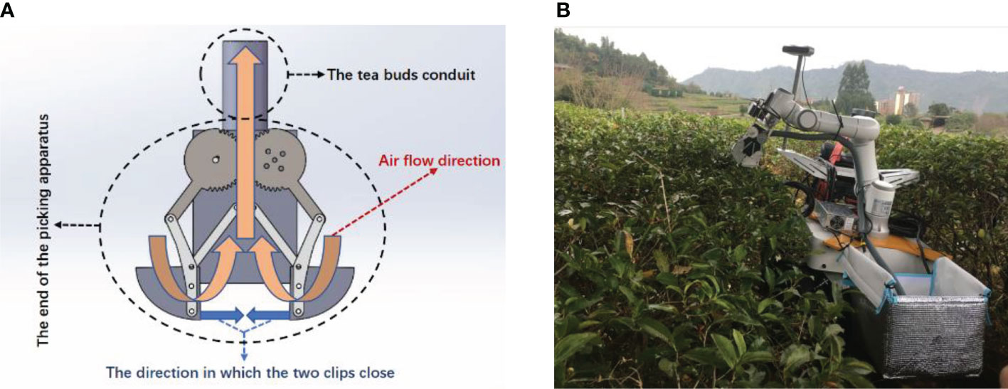
Figure 1 The picking robot and the end of the bud picker. (A) Structural diagram of the end of the bud picker. (B) The picking robot in the field.

The movement of the end of the bud picker can be adjusted by XYZ and θ. The manipulators move the end of the bud picker to a small picking area in the XYZ spatial coordinate and adjust its height according to the depth of the tea ridges. In the picking area, the surfaces of the tea ridges can be set to be flat under the same height. Meanwhile, the consumed time and the lost energy during the picking process are mainly caused by the movement of the end of the bud picker in the XOY plane. For convenience, we only consider the picking path planned in the XOY plane.

When the end of the bud picker moves to a picking area, the foothold parameters of a picking box are fine-tuned to complete a picking. After all buds in the picking area have been picked and collected, the manipulator drives the end of the picker to the next picking area to repeat the action. The picking scheme is divided into three steps: 1) Solving the optimal coverage picking box set, i.e., covering all of the buds in a picking area with the least number of picking box sets and obtaining the foothold parameters of each picking box; 2) Fine-tuning the foothold parameters of each picking box in the optimal coverage picking box set, so that the buds can be concentrated in the picking box as much as possible; 3) According to the foothold parameters of each picking box in the optimal coverage picking box, the end of the bud picker is planned for the shortest picking path. Figure 2 shows the specific picking process.

FIGURE 2

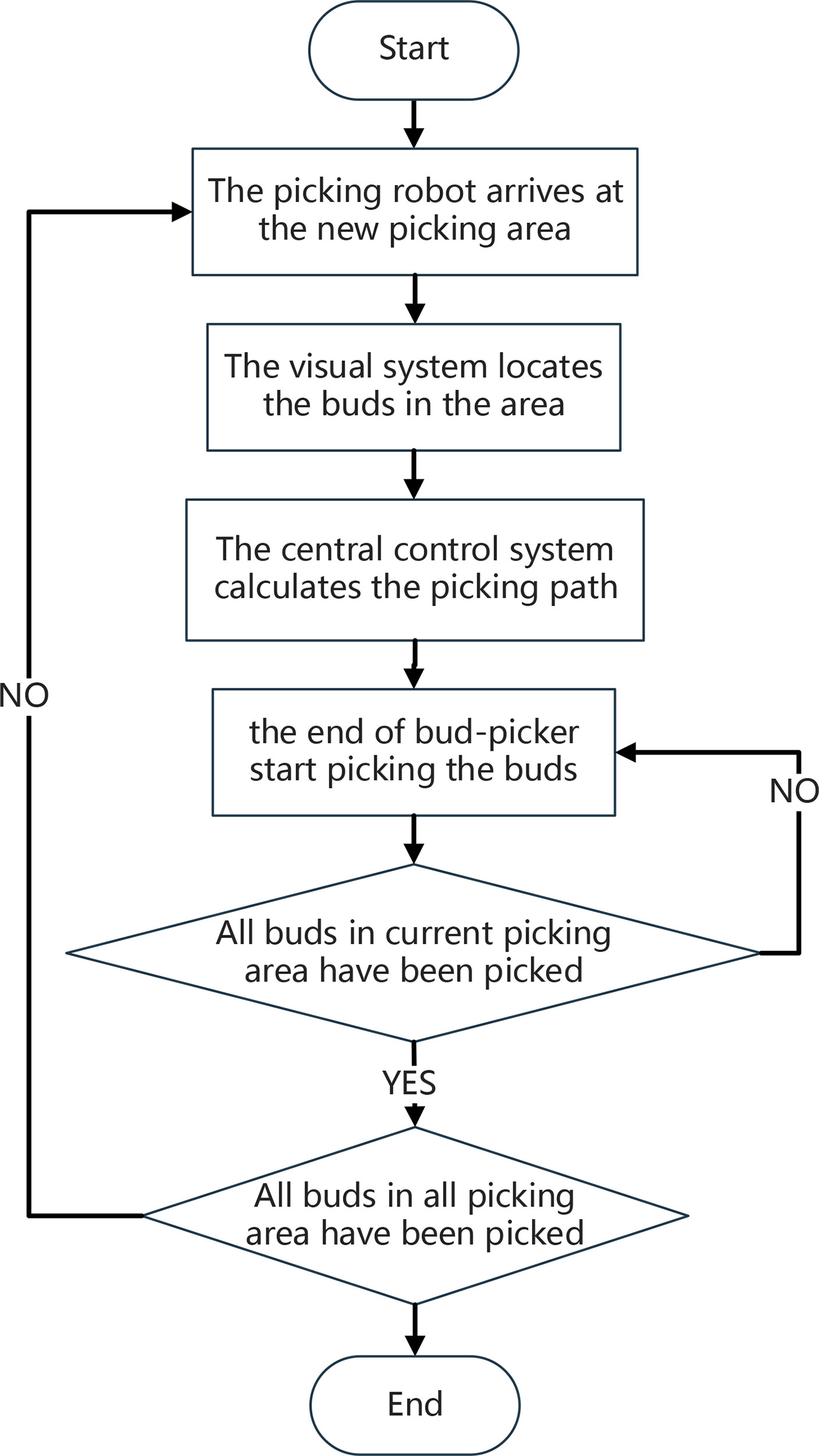
Figure 2 The working flowchart of the picking robot.

Mathematical model of the end of the bud picker

Picking area

In the tea garden of Mingshan district, Ya’an city, Sichuan province, the actual typical distribution of the buds on the tea ridge is shown in Figure 3A. In a small picking area, 50 buds are randomly generated according to the natural distribution and numbered in sequence, as shown in Figure 3B. In the actual experiment, multiple areas are selected for testing, and Figure 3 is just one of them. The length and the width of the picking area are set as 100 and 50 cm, respectively, and the ratio of the length to the width is 2:1, which basically conforms to the natural situation. Furthermore, for convenience, we have simplified the parameters as shown in Table 1.

FIGURE 3

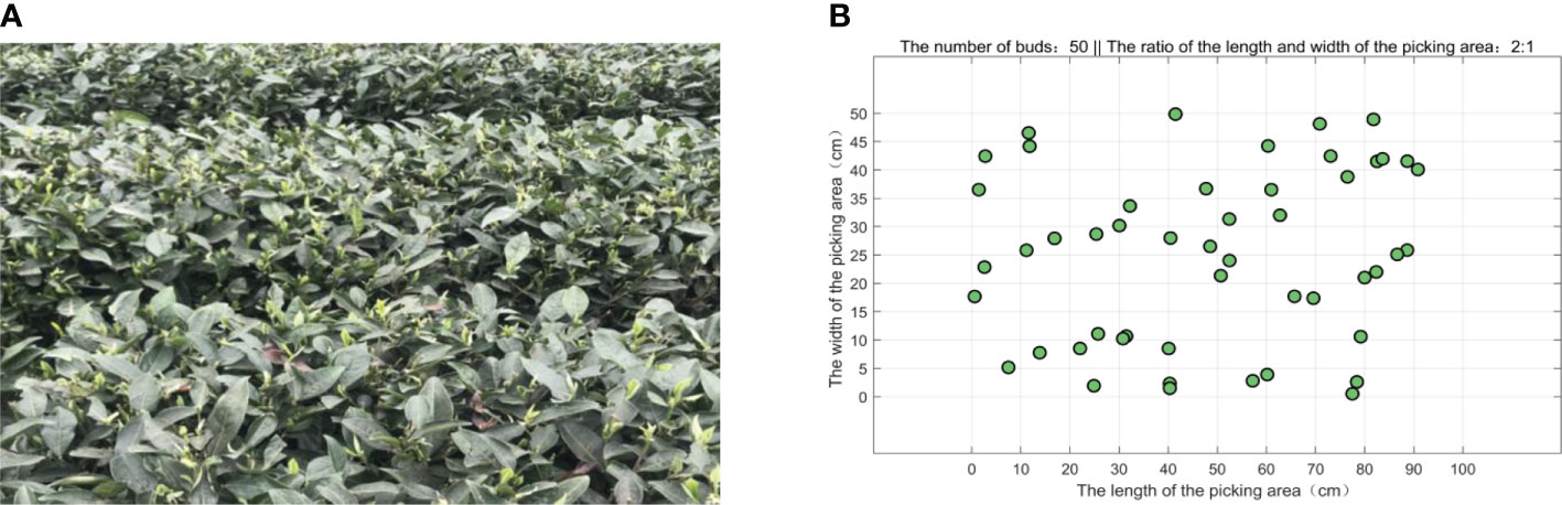
Figure 3 The distribution of the tea buds in a picking area. (A) The actual distribution of the buds in the field. (B) The simulated distribution of 50 buds in a picking area.

TABLE 1

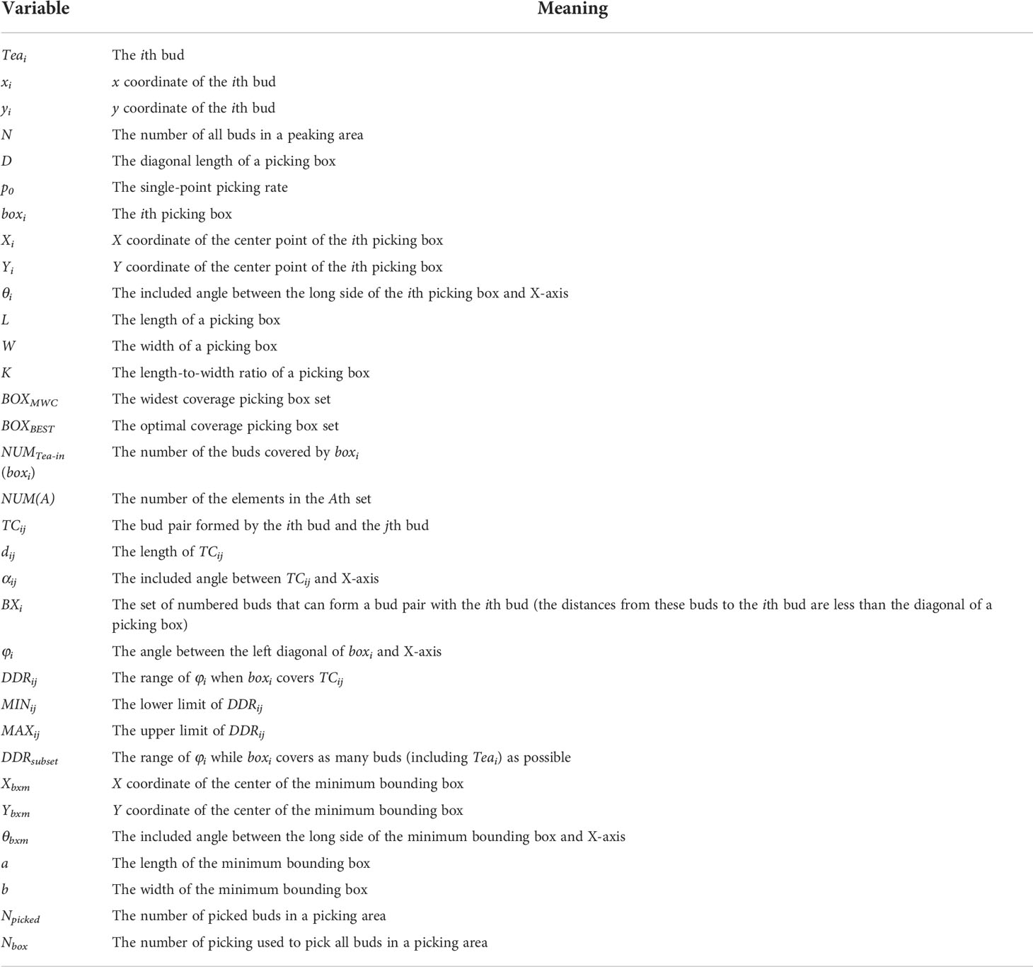
Table 1 Notations.

Picking box

In order to minimize the specific structure of the end of the bud picker and focus on the impact of the end of the picking effect, we abstracted it mathematically and proposed a simplified model of the end of the bud picker with the structure in Figure 4, which was named the picking box. L is the length of the clamping finger, and W is the maximum opening of two clamping fingers. (X_i,Y_i) are the center coordinates of the ith picking box. θ_i is the deflection angle in the coordinate of the picking box (i.e., the included angle between the long side of the ith picking box and X-axis), denoted by the ith picking box as box_i(X_i,Y_i,θ_i,L,W) and briefly as box_i. p₀ is the single-point picking rate, and the parameters such as (X_i,Y_i,θ_i) are the foothold parameters of box_i. (x_i,y_i) are the coordinates of the ith bud in box_i, which are within the range of Line1~Line4 in Figure 4.

FIGURE 4

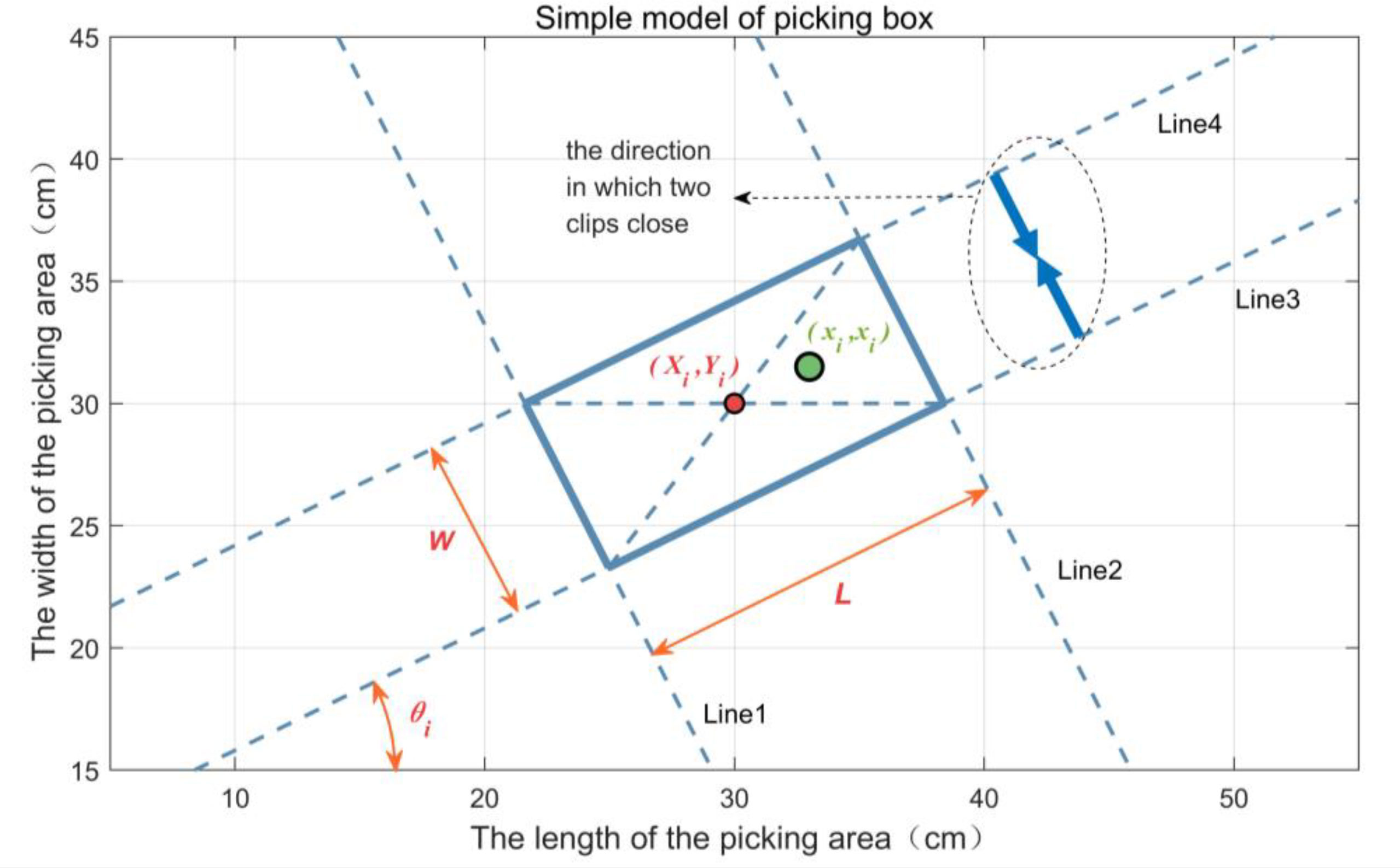
Figure 4 The picking box of the end of a bud picker.

In Figure 4, the mathematical model of a picking box is as follows:

$\begin{array}{ll}\{\begin{array}{l}\begin{array}{c}\left|y_i-\tan {\theta }_i(x_i-X_i)-Y_i\right|\le \frac{W}{2\cos {\theta }_i}\\ \left|y_i+\frac{1}{\tan {\theta }_i}(x_i-X_i)-Y_i\right|\le \frac{L}{2\sin {\theta }_i}\end{array} \},{\theta }_i\in -\text{π},\text{π}],{\theta }_i\ne \frac{k\text{π}}{2},k\in \{-2,-1,0,1,2\}\hfill \\ \begin{array}{l}|x_i-X_i|\le \frac{L}{2}\hfill \\ |y_i-Y_i|\le \frac{W}{2}\hfill \end{array}\},{\theta }_i=\frac{k\text{π}}{2},k\in \{-2,0,2\}\hfill \\ \begin{array}{l}|x_i-X_i|\le \frac{W}{2}\hfill \\ |y_i-Y_i|\le \frac{L}{2}\hfill \end{array}\},{\theta }_i=\frac{k\text{π}}{2},k\in \{-1,0,1\}\hfill \end{array}& (1)\end{array}$

where i = 1, …, N (N is the number of all buds in a picking area).

Equation 1 means that the ith bud can be picked by box_i(X_i,Y_i,θ_i,L,W) with the probability of p₀, and the probability of each bud being picked is equal to and independent of each other:

$\begin{array}{ll}Tea(x_i,y_i)\stackrel{p_0}{\to }box(X_i,Y_i,{\theta }_i,L,W)& (2)\end{array}$

Alternatively, briefly as:

$\begin{array}{ll}Te{a}_i\stackrel{p_0}{\to }bo{x}_i& (3)\end{array}$

The optimal coverage picking box set BOX_BEST

The combined multipoint picking scheme is as follows:

1) Traverse the ith bud and use it as a reference point to solve box_i. box_ican certainly cover the ith bud and cover as many other buds as possible, thus the widest coverage picking box set BOX_MWC can be constructed as:

$\begin{array}{ll}BO{X}_{MWC}=\left\{bo{x}_i\right|i=1,2,3\dots N\}& (4)\end{array}$

where BOX_MWC means that each bud can be covered by at least one picking box ^] (Wei and Han, 2016), and the picking box can cover as many other buds as possible. The picking boxes in BOX_MWC should meet the following conditions:

$\begin{array}{ll}\{\begin{array}{l}\underset{bo{x}_i}{\max }\hspace{0.17em}NU{M}_{Tea-in}(bo{x}_i)\hfill \\ s.t.Te{a}_i\stackrel{p_0}{\to }bo{x}_i\hfill \end{array}& (5)\end{array}$

where NUM_{Tea – in}(box_i) is the number of the buds covered by box_i.

2) Use the greedy algorithm to select the optimal coverage picking box set BOX_BEST from BOX_MWC to minimize the number of picking boxes, and BOX_BEST can cover all buds in a picking area:

$\begin{array}{ll}BO{X}_{BEST}\subset BO{X}_{MXC}& (6)\end{array}$

This means that BOX_BEST is a subset of BOX_MWC.

The constraint condition is described as follows:

$\begin{array}{ll}\{\begin{array}{l}\underset{CU{T}_{BEST}}{\min }NUM(BO{X}_{BEST})\hspace{0.17em}\hfill \\ s.t.\hspace{1em}NU{M}_{Tea-in}(BO{X}_{BEST})=N\hfill \\ \hspace{1em}L,W=Constant\hfill \end{array}& (7)\end{array}$

where NUM_{Tea – in}(BOX_BEST) is the number of the buds covered by BOX_BEST.

Solution of BOX_MWC

Constructing the bud pairs

A bud pair refers to two buds that can be picked together at one time by the end of the bud picker, and it is a reference point for selecting the foothold parameters of each picking box. Then, the BOX_MWC is solved. To obtain box_i of the ith bud, two-point picking needs to be solved first. Given that the diagonal length of box_i is D when the ith bud and the jth bud can be picked together, the constraint condition is as follows:

$\begin{array}{ll}{d}_{ij}\le D& (8)\end{array}$

Then, a directed line segment is constructed, and it is recorded as a bud pair TC_ij:

$\begin{array}{ll}T{C}_{ij}=(d_{ij},{\alpha }_{ij})& (9)\end{array}$

where

$\begin{array}{ll}{d}_{ij}=\sqrt{{(x_i-x_j)}^2+{(y_i-y_j)}^2}& (10)\end{array}$

$\begin{array}{ll}{\alpha }_{ij}=\{\begin{array}{l}\arctan \left(\frac{y_j-y_i}{x_j-x_i}\right),x_i\ne x_j\hfill \\ \frac{\text{π}}{2},x_i=x_j\hspace{0.17em}and\hspace{0.17em}{y}_i\ge y_j\hfill \\ -\frac{\text{π}}{2},x_i=x_j\hspace{0.17em}and\hspace{0.17em}{y}_i<y_j\end{array}& (11)\end{array}$

where α_ij∈(−π,π) is the angle between TC_ij and X-axis.

All of the buds are gone through to form bud pairs and are numbered. The ith bud is taken as an example, its alternative bud set is named BX_i, in which each bud can be formed into a bud pair with the ith bud. The buds in BX_i can be covered by box_i:

$\begin{array}{ll}B{X}_i=\left\{j\right|d_{ij}\le D\}& (12)\end{array}$

When D is set as $2\sqrt{10}$cm with L = 6 cm and W = 2 cm, the bud pairs can be constructed from Figure 1 as shown in Figure 5. From Figure 5, we know that there are 25 pairs of buds in a picking area.

FIGURE 5

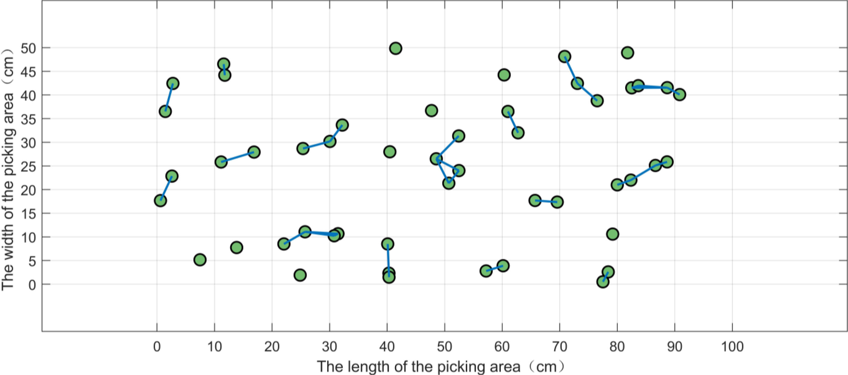
Figure 5 The bud pairs.

Solution of foothold parameters of box_i

According to Equation 1, when the length L and the width W of box_i have been determined, its foothold parameters (X_i,Y_i,θ_i) have not yet been confirmed. If the enumeration judgment is traversed with a certain accuracy of (ΔX, ΔY, Δθ), the time complexity of algorithm is up to O (n³). However, if there are too many buds, the high-speed decision requirement cannot be met. To solve this problem, the starting point of TC_ijis taken as the circle center, which coincides with the lower left vertex of box_i. The angle between the left diagonal of box_i and X-axis is denoted by φ_i when TC_ij is covered by box_i, and the maximum value of φ_i is denoted as MAX_ij. Similarly, the minimum value of φ_i is denoted as MIN_ij. Under different values of d_ij, MIN_ij and MAX_ij, formed by the rotating action of box_i, are shown in Figure 6.

FIGURE 6

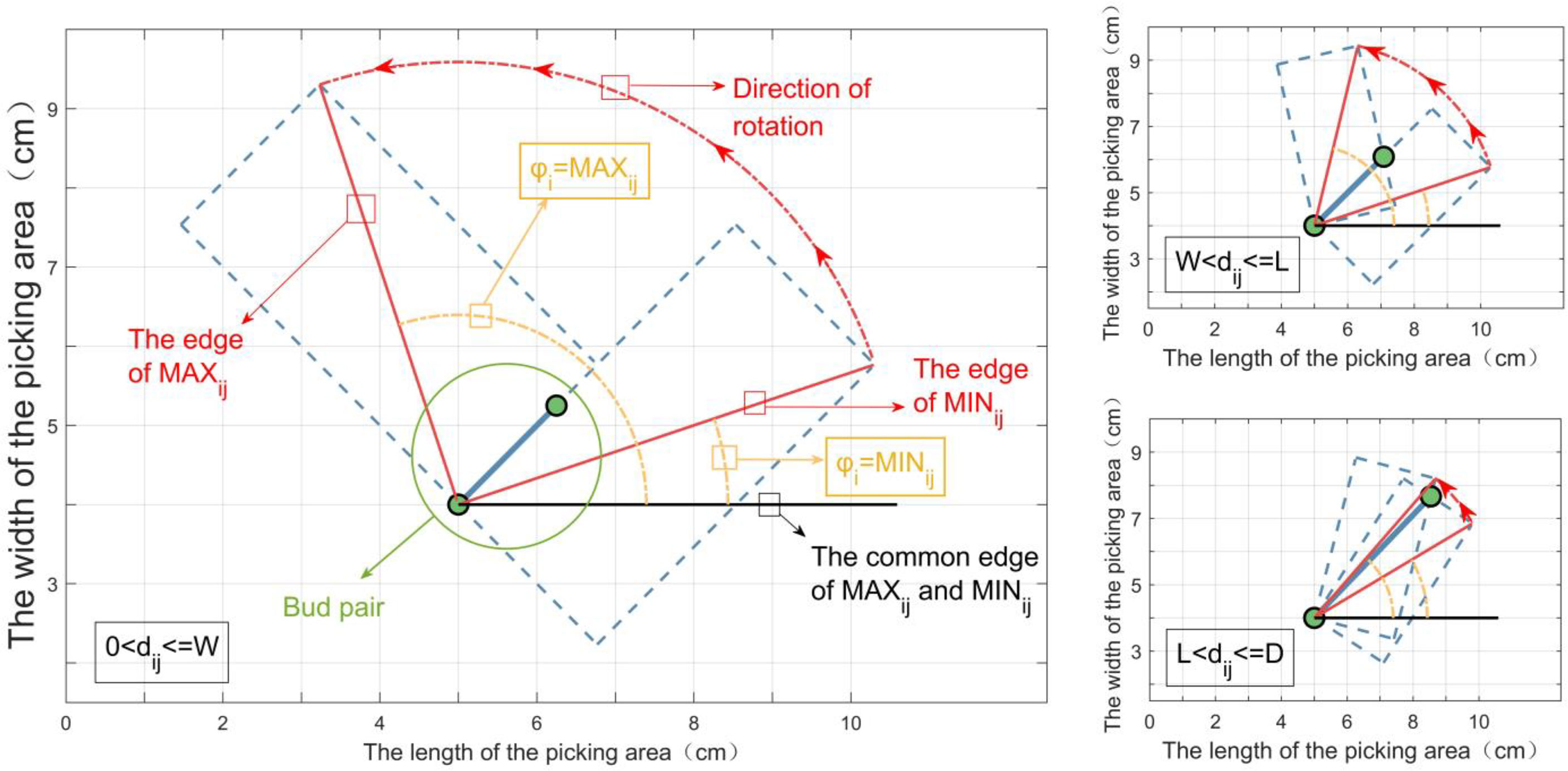
Figure 6 The minimum/maximum angles formed by the rotating action of box_i..

According to geometric knowledge, we have the following:

$\begin{array}{ll}\begin{array}{l}MI{N}_{ij}=\{\begin{array}{l}{\alpha }_{ij}-\arctan \left(\frac{W}{L}\right)\hspace{0.17em}{d}_{ij}\le L\hfill \\ {\alpha }_{ij}+\arccos \left(\frac{L}{d_{ij}}\right)-\arctan \left(\frac{W}{L}\right)d_{ij}>L\hfill \end{array}\hfill \\ MA{X}_{ij}=\{\begin{array}{l}{\alpha }_{ij}+\arctan \left(\frac{W}{L}\right)\hspace{0.17em}{d}_{ij}\le W\hfill \\ {\alpha }_{ij}-\arccos \left(\frac{L}{d_{ij}}\right)+\arctan \left(\frac{W}{L}\right)d_{ij}>W\hfill \end{array}\hfill \end{array}& (13)\end{array}$

According to Equation 13, the rotation range of the left diagonal of box_i can be obtained, and it is denoted as follows:

$\begin{array}{ll}DR{R}_{ij}=[MI{N}_{ij},MA{X}_{ij}]& (14)\end{array}$

For two bud pairs such as TC_ij1 and TC_ij2 with the same starting point (where the j₁th bud and the j₂th bud∈BX_i), they can be picked together by the box_i when DRR_ij1 and DRR_ij2 have an intersection. If a subset A of the set {DRR_ij|j∈BX_i} can be found with the most elements and all elements in A have a common non-empty intersection DRR_subset, the box_i can cover as many buds as possible including the reference bud Tea_i. It is transformed into the following optimization problem:

$\begin{array}{ll}\{\begin{array}{l}\underset{DR{R}_{subset}}{\max }\hspace{0.17em}NUM(A)\hfill \\ s.t.\hspace{0.17em}\hspace{0.17em}A\subset \left\{DR{R}_{ij}\right|j\in B{X}_i\}\hfill \\ \hspace{1em}\underset{k=1}{\overset{NUM(A)}{\cap }}A(k)=DR{R}_{subset}\hfill \\ \hspace{1em}DR{R}_{subset}\ne \varnothing \hfill \end{array}& (15)\end{array}$

where A(k) is the kth element of A.

By randomly selecting φ_i, the foothold parameters (X_i,Y_i,θ_i) of box_i corresponding to Tea_i can be obtained, which are calculated as follows:

$\begin{array}{ll}\{\begin{array}{l}{X}_i=\frac{1}{2}D·\cos ({\theta }_i)+x_i\hfill \\ Y_i=\frac{1}{2}D·sin({\theta }_i)+y_i\hfill \\ {\theta }_i={\phi }_i+\arctan \left(\frac{W}{L}\right)\hfill \end{array}& (16)\end{array}$

Furthermore, DRR_subset can be solved by the interval scanning method below.

As shown in Figure 7, suppose that there is a detector (i.e., the red vertical solid line in Figure 7) that scans counterclockwise with a certain step length. When it intersects the DRR_ij (i.e., the blue horizontal solid line in Figure 7, j = 1,2,…,10), it is marked as a detection point (i.e., the red square in Figure 7) at the intersection. Each time the detector moves, the detection point is counted once. When the number of detection points increases, the lower limit of DRR_subset is updated to the α-axis coordinate of the position of the detector; when the number of detection points does not change, the upper limit of DRR_subset is updated to the α-axis coordinate of the position of the detector; if the number becomes smaller, it will not be updated. After detector scanning for a circle, DRR_subset is recorded as [30⁰, 60⁰] in Figure 6. Foothold parameters (X_i,Y_i,θ_i) of box_i can be calculated for Tea_i, while φ_i takes the middle value of DRR_subset. Using the same way to traverse each bud, the widest coverage picking box set BOX_MWC can be obtained finally.

FIGURE 7

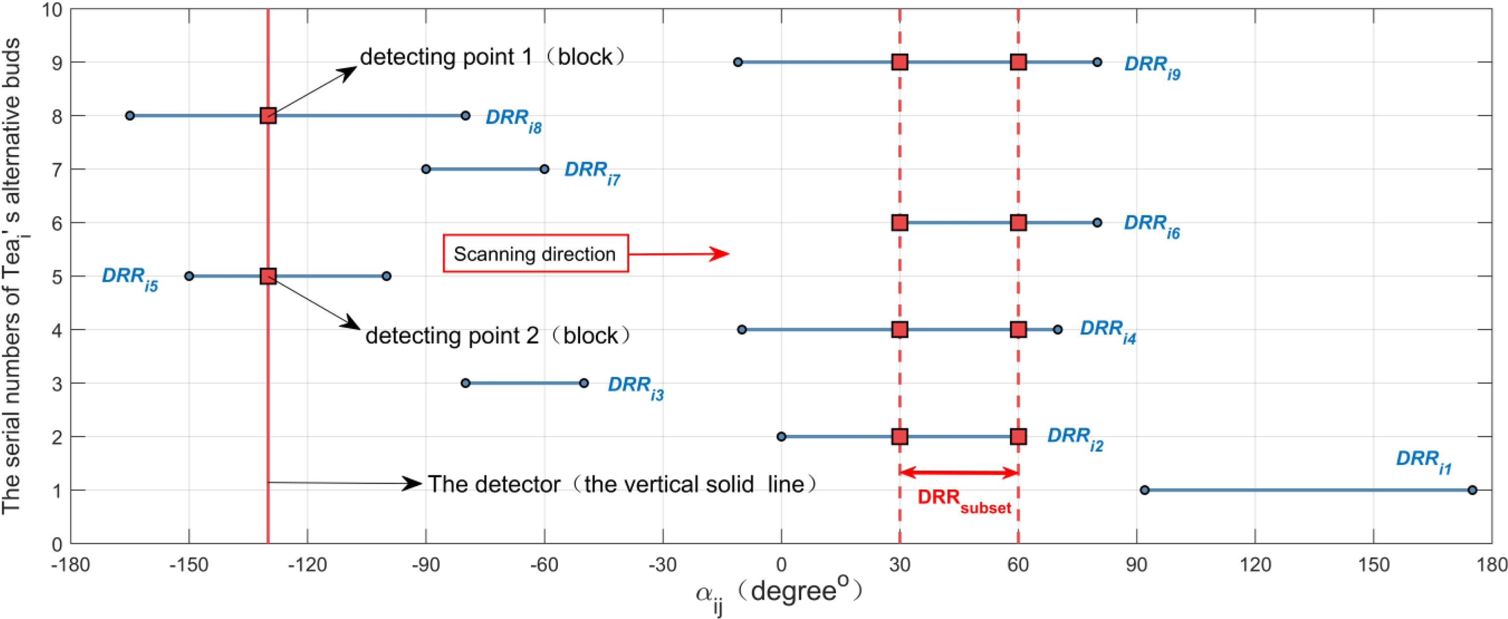
Figure 7 Schematic diagram of the interval scanning method.

Foothold parameters (X_i,Y_i,θ_i) of box_i calculated by the above method are not necessarily a globally optimal solution. As shown in Figure 8, the inner angles of the convex hull of the point set formed by the reference bud (i.e., Tea_i1 or Tea_i2 shown in Figure 8) and its alternative buds (i.e., {Tea_j1|j₁∈BX_i1} or {Tea_j2|j₂∈BX_i2} ) that can be picked together are greater than 90°, which will lead to local optimums. No matter how box_i rotates, it cannot cover all buds. If the inner angle of the convex hull of the point set formed by the imaginary reference bud in Figure 8 and its alternative buds is not more than 90⁰, the ideal box_i can cover all buds, which means that foothold parameters of box_i can be calculated preferably (Cheein and Guivant, 2014; Gao et al., 2015).

FIGURE 8

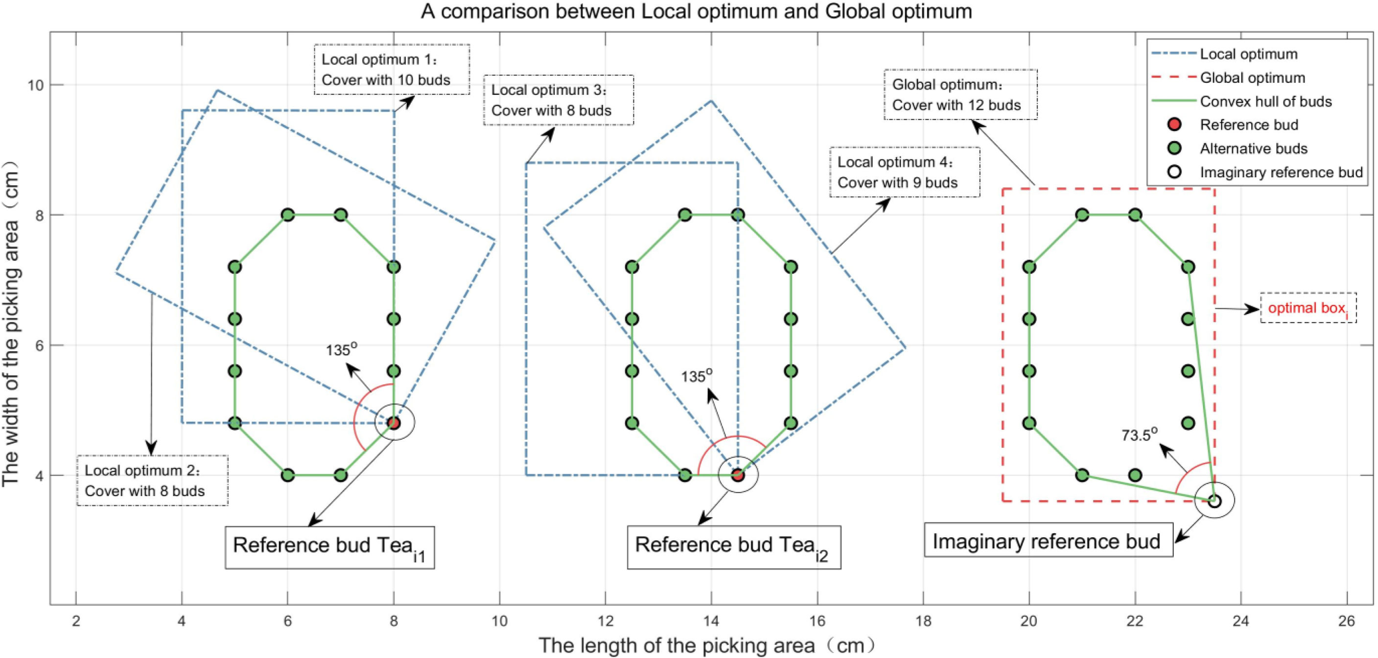
Figure 8 Comparison of local optimum and global optimum.

As shown in Figure 8, although the probability that the inner angles are greater than 90⁰ is extremely small in fact, the opposite situation still happens (i.e., Tea_i1 or Tea_i2 shown in Figure 8) occasionally, in which the buds can be covered by two picking boxes. This situation only uses one more picking box than ideal. In Figure 8, the third and fourth local optimums of box_i are superimposed to completely cover 12 buds to be picked. Therefore, the above method is sufficient to meet the actual picking demand.

Solution of BOX_BEST

BOX_BEST means to cover all buds in a picking area with the least number of picking boxes. According to Equation 6, BOX_BEST is a subset of BOX_MWC. To traverse each box_i in BOX_MWC, use Equation 1 to find the buds covered by box_i, record their numbers, and finally establish a bud set HC_i as follows:

$\begin{array}{ll}H{C}_i=\left\{j\right|Te{a}_j\stackrel{p_0}{\to }bo{x}_i\},i=1,\cdots ,N& (17)\end{array}$

The greedy algorithm is used to obtainCUTBESTand the steps are as follows (Tong et al., 2017; Zhao et al., 2017; Zhang et al., 2018). Firstly, find the set with the most elements in HC_i(i=1,2,…N) and record its subscript i_most. Secondly, remove all elements of the set HC_imost and remove the elements of HC_i (i ≠ i_most) that are also of HC_imost . Thirdly, put box_imost into BOX_BEST. Repeat the above steps until the number of elements in all sets (HC₁,HC₂,…,HC_N) is zero, and then BOX_BEST can be obtained finally. The picking boxes in BOX_BEST are shown in Figure 9.

FIGURE 9

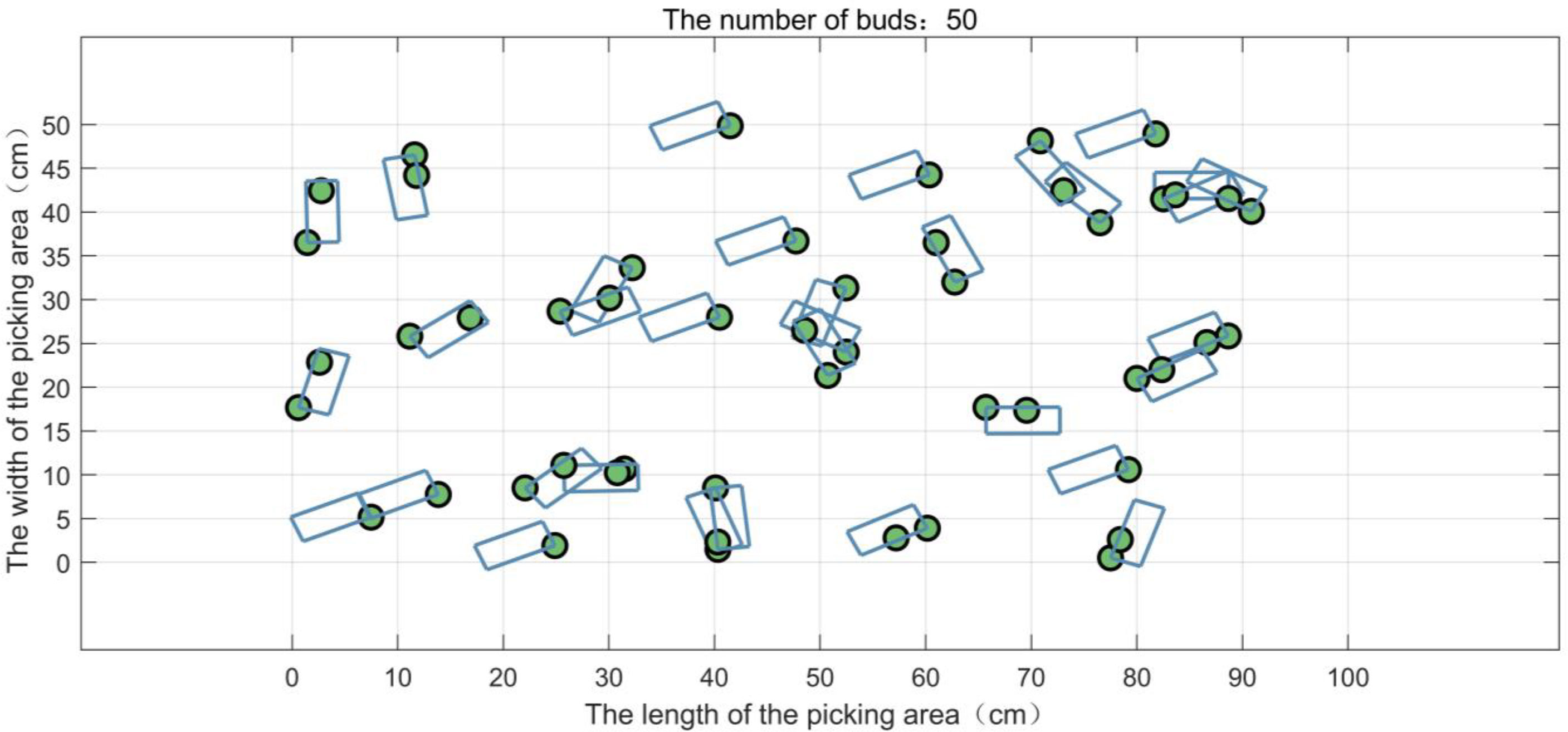
Figure 9 The picking boxes in BOX_BEST (before fine-tuning).

Fine-tuning the foothold parameters of picking boxes in BOX_BEST

BOX_BEST essentially classifies all buds, and the buds that can be covered by the same picking box are classified into one category. Figure 9 shows that many buds are on the edges of the picking boxes, so it is necessary to fine-tune the foothold parameters of picking boxes in BOX_BEST to make the most buds concentrated in the middle of the picking boxes as much as possible and thus ensure the integrity of buds after being picked together.

For the bud set covered by a picking box in BOX_BEST, use the Graham algorithm to solve the convex hull of the bud set (Song et al., 2012; Zhang et al., 2019) and then apply the convex hull to calculate the minimum bounding box of the bud set (Park and Lim, 2014; Tang et al., 2018). The central coordinate of the minimum bounding box is (X_bxm,Y_bxm), and the angle between the long side of the minimum bounding box and X-axis is θ_bxm. The length and width of the minimum bounding box are a and b, respectively. Then, (X_bxm,Y_bxm,θ_bxm) are the fine-tuned foothold parameters of each picking box inBOX_BEST, and a b meet the following constrained conditions:

$\begin{array}{ll}\{\begin{array}{c}\underset{a,b}{\min }ab\\ \begin{array}{ccc}s.t.& a\le L,& b\le W\end{array}\end{array}& (18)\end{array}$

According to Cheng et al. (2008), if a point set has the minimum bounding box, an edge of its minimum bounding box must coincide with an edge of its convex hull. By this, traverse each edge l_k(k = 1,2,…,n) of the convex hull, then take l_k as the reference edge, and make the circumscribed rectangle of the point set, so that one edge of the rectangle coincides with l_k, and the parameters of the rectangle can be obtained by geometric knowledge. A set of parameters satisfying the condition of Equation 18 is the parameter (X_bxm,Y_bxm,θ_bxm,a,b) of the minimum bounding box (Yan et al., 2013).

Taking a randomly distributed bud set of eight buds as an example, the convex hull of the point set obtained by the Graham algorithm is shown in Figure 10A, and the minimum bounding box of the bud set is shown in Figure 10B.

FIGURE 10

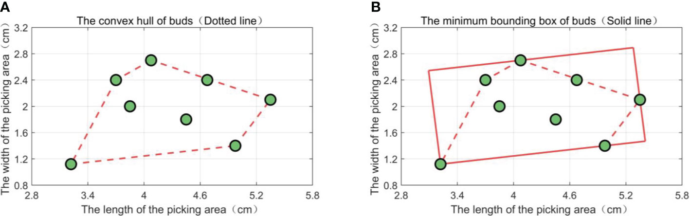
Figure 10 Convex hull of the bud set and its minimum bounding box. (A) A diagram of the convex hull of a point set. (B) A diagram of the minimum bounding box of a point set.

The parameters (X_bxm,Y_bxm,θ_bxm) of the minimum bounding box are obtained as the fine-tuned foothold parameters of the corresponding picking box in BOX_BEST. The position comparison before and after the fine-tuning of the picking box’s footing point parameters is shown in Figure 11. From Figure 11, it can be seen that the buds are concentrated in the middle of the fine-tuned picking box.

FIGURE 11

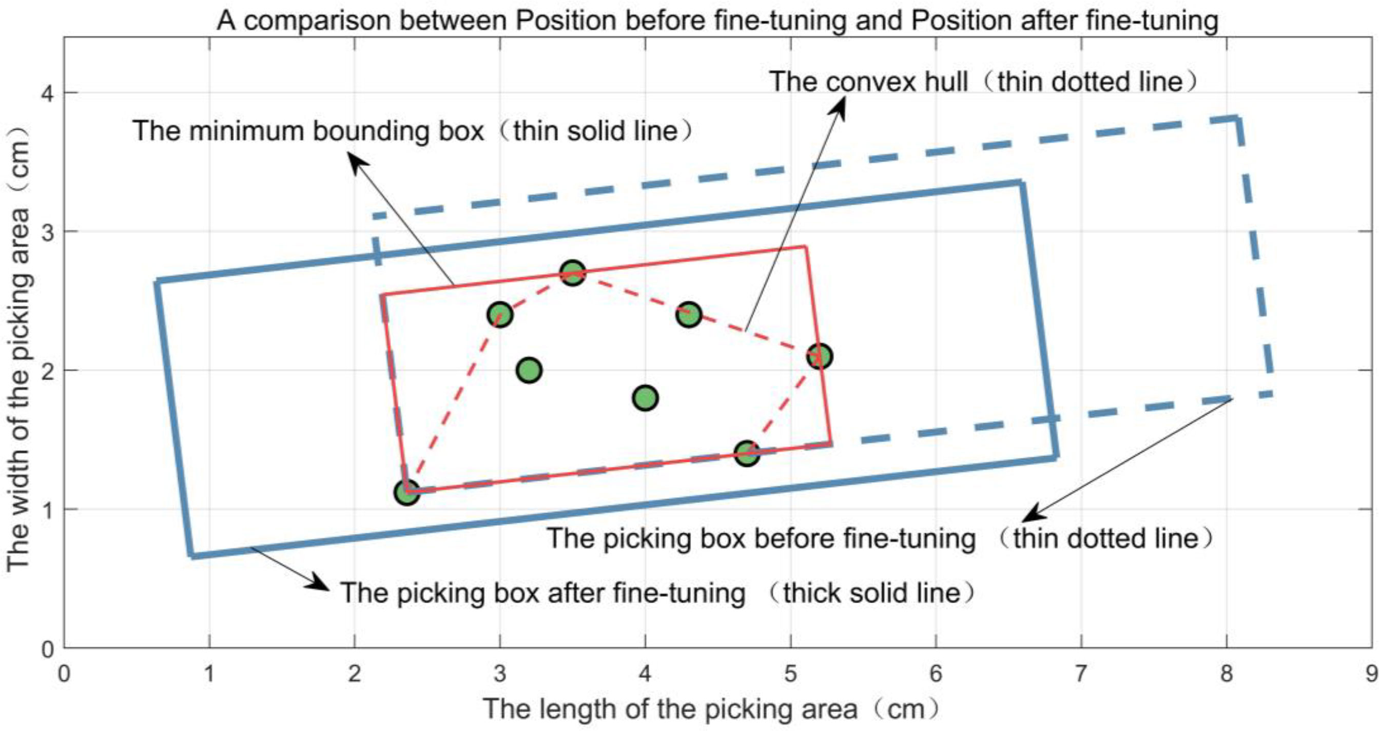
Figure 11 Position comparison of a picking box before and after fine-tuning its foothold parameters.

Results and discussion

Solving the shortest path

The optimal foothold parameters of a picking box (i.e., the end of the bud picker) have been obtained in the foregoing. In order to further improve the picking efficiency, the ant colony algorithm is applied to plan the optimal picking path of the end of the bud picker (Jiang et al., 2015; Wang et al., 2020; Lin et al., 2020). The information track persistence parameter is adaptively changed (Wen et al., 2017; Deng et al., 2018; Wang L. et al., 2018), and the other parameters of the ant colony algorithm are screened out after many experiments (see Table 2 for details).

TABLE 2

Table 2 Parameters of the ant colony algorithm.

When the end of the bud picker moves on the XOY plane, its rotation angle θ can be adjusted synchronously. When planning the picking path with the goal of shortening the consumed time, the adjusting time of θ can be ignored, and it is regarded as planning the picking path of the manipulator in the XOY plane. Set the length L = 6 cm and the width W = 2 cm of a picking box for simulation. The CPU is the Intel core i5-6300HQ processor with the memory capacity of 4 GB. The results of the single-point picking scheme (abbreviated as SPS) and the combined multipoint picking scheme (abbreviated as CPS) are shown in Figure 12.

FIGURE 12

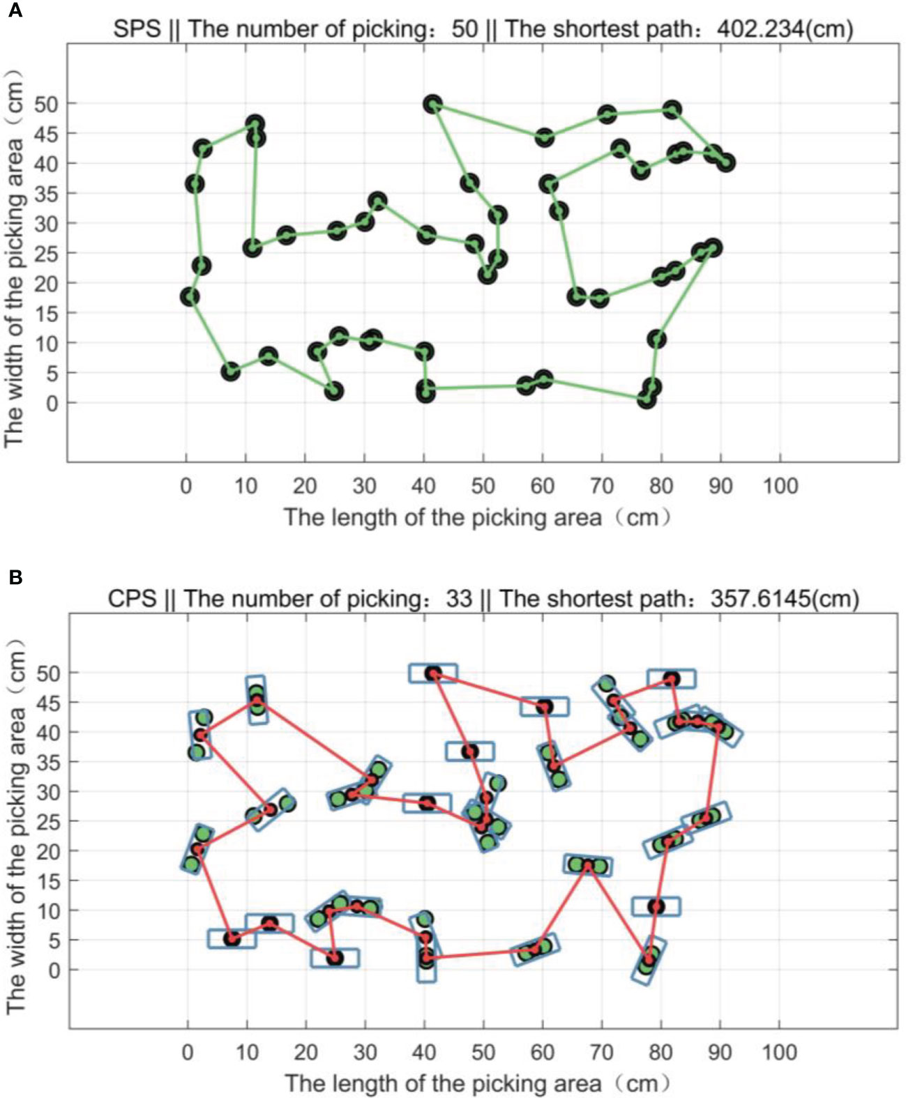
Figure 12 The shortest paths of two picking schemes. (A) The shortest paths of the single-point picking scheme (SPS). (B) The shortest paths of the combined multipoint picking scheme (CPS).

In a picking area, 50 buds are randomly distributed 100 times, and the experiment is repeated. Experimental results of the two picking schemes are shown in Figure 13, and the statistical results are listed in Table 3.

FIGURE 13

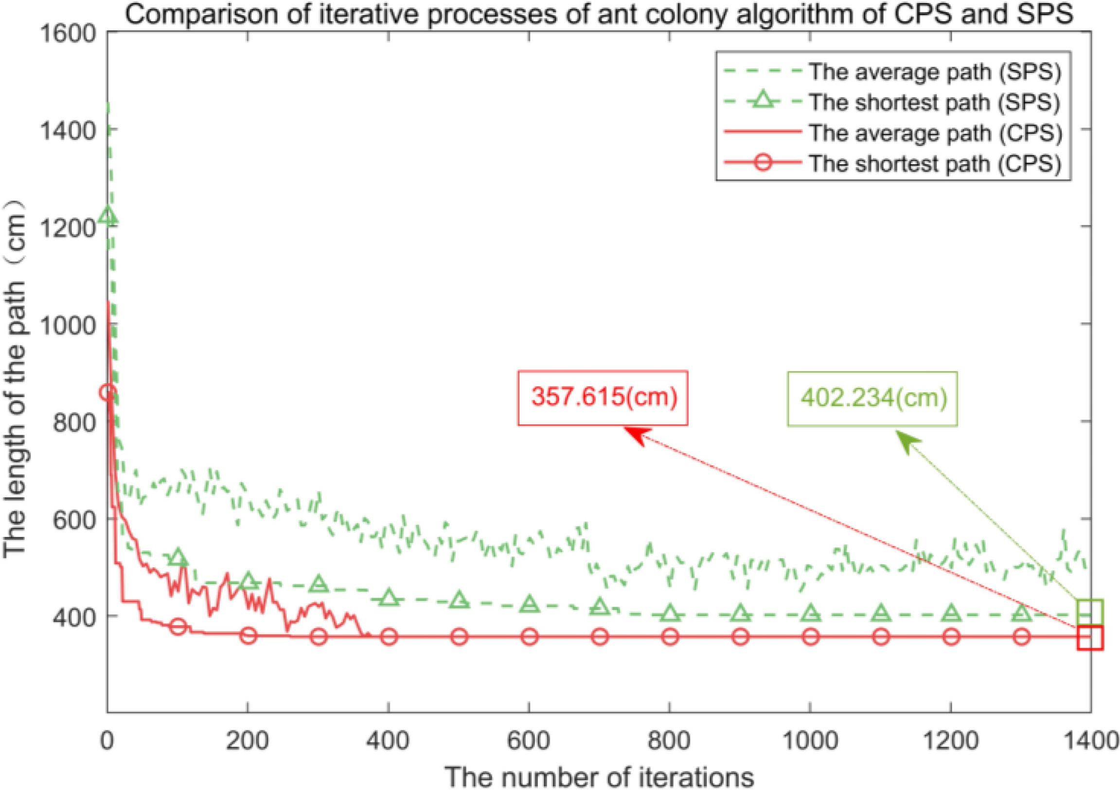
Figure 13 Comparison of the average shortest picking path and the shortest picking path of the two picking schemes.

TABLE 3

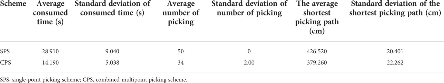
Table 3 Comparison of 100 experimental statistical results of the two picking schemes.

From Figures 12, 13 and the data in Table 3, it can be seen that all buds are in the middle of the picking boxes and 1–2 buds can be picked successfully at a time. Compared with the SPS, the average number of picking of the CPS is reduced by 31.44%, the shortest picking path is decreased by 11.10%, and the average consumed time is reduced by 50.92%, so its picking performance is better than that of the SPS.

The data in Table 3 were tested by the Z hypothesis test to analyze the significant differences between the two schemes in terms of the consumed time, the number of picking, and the shortest picking path. The Z-test was calculated as follows:

$\begin{array}{ll}Z=\frac{\left|\overline{X_{SPS}}-\overline{X_{CPS}}\right|}{\sqrt{\frac{S_{SPS}^2}{n_{ex}}+\frac{S_{CPS}^2}{n_{ex}}}}& (19)\end{array}$

where $\overline{X_{SPS}}$ and $\overline{X_{CPS}}$ are the mean values of the specific data in the SPS scheme and the CPS scheme, respectively, S_SPS and S_CPS are the standard deviations of the specific data in the SPS scheme and the CPS scheme, respectively, and n_ex is the number of experiments that is set to 100。.

According to the hypothesis test table, when Z is greater than 1.96, it is corresponding to the significance P ≤ 0.05, which indicates that there is a significant difference between the two schemes under this parameter. According to Equation 19, Z equals 14.22, 80.00, and 15.65 for the consumed time, the number of picking, and the shortest picking path, respectively; therefore, there are significant differences between the two schemes in the abovementioned three parameters.

Evaluating the scheme under different parameters

Setting the range of parameters

If the L, W, p₀, and N are different, the N_picked and N_box will be different, as follows:

$\begin{array}{ll}[N_{picked},N_{box}]=f(L,W,p_0,N)& (20)\end{array}$

In order to analyze the effect of the above four parameters on the performance of the CPS scheme and optimize it, a factorial design is adopted. Different steps and ranges are set for the parameters including L, W, p₀, and N in Table 4. Each group of four parameters is used in the procedure 50 times to calculate the average value. A total of 10,000 pairs of [N_picked, N_box] can be obtained.

TABLE 4

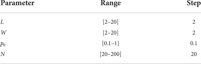
Table 4 Parameter setting.

In order to obtain more accurate quantized parameters, the level number was set to 10, which will increase the difficulty of parameter analysis. Therefore, targeted analysis was made on the part of experimental results that help optimize the CPS scheme.

Evaluation indicator

Three indicators, Δp (i.e., the increment of total picking rate), Δr (i.e., the reduction ratio of the number of picking), and Q (i.e., the yield per unit area), are used to evaluate the performance of the picking scheme.

1) Δp. The CPS will cause a probability of repeatedly picking a bud. Δp is the increment of total picking rate of the CPS compared to that of the SPS. Δp is calculated as follows:

$\begin{array}{ll}\Delta p=\frac{N_{picked}}{N}-p_0& (21)\end{array}$

$\begin{array}{ll}{N}_{picked}=N-{\displaystyle \sum _{i=1}^N{(1-p_0)}^{m_i}}\hspace{0.17em}& (22)\end{array}$

where m_i is the number that the ith bud is repeatedly picked.

2) Δr. The less the number of picking in a picking area, the shorter the picking path. Δr is the reduction ratio of the number of picking of the CPS compared to that of the SPS. Δr is calculated as follows:

$\begin{array}{ll}\Delta r=\frac{N-N_{box}}{N}& (23)\end{array}$

3) Q. The smaller the area of the picking box, the higher the integrity rate of the picked buds. p₀ will decrease with the increase of S. That is, the smallest area of a picking box can get the maximum values of Δp and Δr. Q is calculated as follows:

$\begin{array}{ll}Q=\frac{\Delta p\Delta r}{S}& (24)\end{array}$

where S is the area of a picking box.

When Q is the maximum value, the corresponding L and W are the optimal sizes of a picking box. It should be noted that Δp = 0 when p₀ = 1, the overall picking rate will no longer increase, and Q = 0 at this time. In order to evaluate the yield under the special case of p₀ = 1, a new evaluation model is constructed as follows:

$\begin{array}{ll}{Q}_r=\frac{\Delta r}{S}& (25)\end{array}$

where Q_r is the yield per unit area, while p₀ = 1. That is, if the performance of the end of the bud picker is optimal, Q is usually used as the evaluating criterion. If the focus is on the improvement of picking efficiency, Q_r will be used as the criterion.

The above indicators are used to select the optimal parameters including the length-to-width ratio and the area of a picking box to achieve the best picking performance under different parameter pairs (N, p₀).

Evaluation analysis on the parameters

1) Influencing factors of Δp and Δr

The relationship between Δp and Δr with the parameters W, L, and N is shown in Figure 14. It can be seen from Figure 14 that when the single-point picking rate p₀ is constant (i.e., p₀ is set as 0.5), Δp (W, L, N) and Δr (W, L, N) are both curved surfaces. When N is constant, Δp and Δr are both increasing with the increase of L and W. When L and W are constant, Δp and Δr are both increasing with the increase of N. The overall picking rate can be increased by about 25%, and the number of picking can be reduced by about 80%.

FIGURE 14

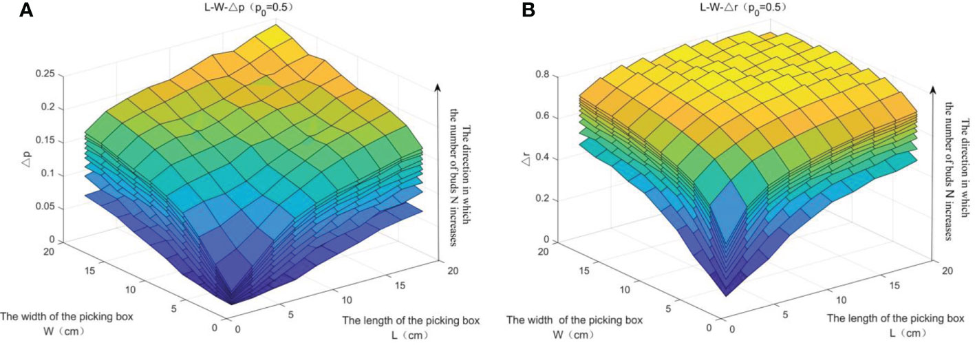
Figure 14 The relationship of Δp and Δr with the parameters W, L, and N. (A) The relationship of Δp with the parameters W, L, and N. (B) The relationship of Δr with the parameters W, L, and N.

2) The influence factors of Q and the selection of the optimal length-to-width ratio of a picking box

The relationship between L, W, and Q is shown in Figure 15. It can be seen from Figure 15 that Q increases with the increase of N, while p₀ is constant (i.e., p₀ = 0.5). With the increase of L and W, Q does not show a monotonous increasing trend, and it is significantly higher in the edge area than in the center area. The top view of Figure 15A is shown in Figure 15B, from which it can be seen that the value of Q in the stripe area of W = 2 is significantly higher than that of other areas, especially when L = 6 or 8, Q reaches the maximum value. Under different values of N and p₀, the experimental results provide a theoretical basis for selecting the optimal length-to-width ratio of a picking box to reach the maximum value of Q.

FIGURE 15

Figure 15 The relationship between L, W, and Q. (A) The relationship between L, W, and Q. (B) The relationship between L, W, and Q (top view).

The influence of K on Q is analyzed with different values of N and p₀. W is set as 2 for simulation, and the results are shown in Figure 16. It can be shown from Figure 16 that K shows a downward trend with the increase of N while Q is the maximum, and the trend has no significant change as p₀ increases from 0.1 to 0.9. When Q or Q_r is the maximum value, the influence of N on K is shown in Figure 16, from which it can be seen that when p₀ = 1, Q_r decreases with the increase of N and then remains stable after N ≥ 60.

FIGURE 16

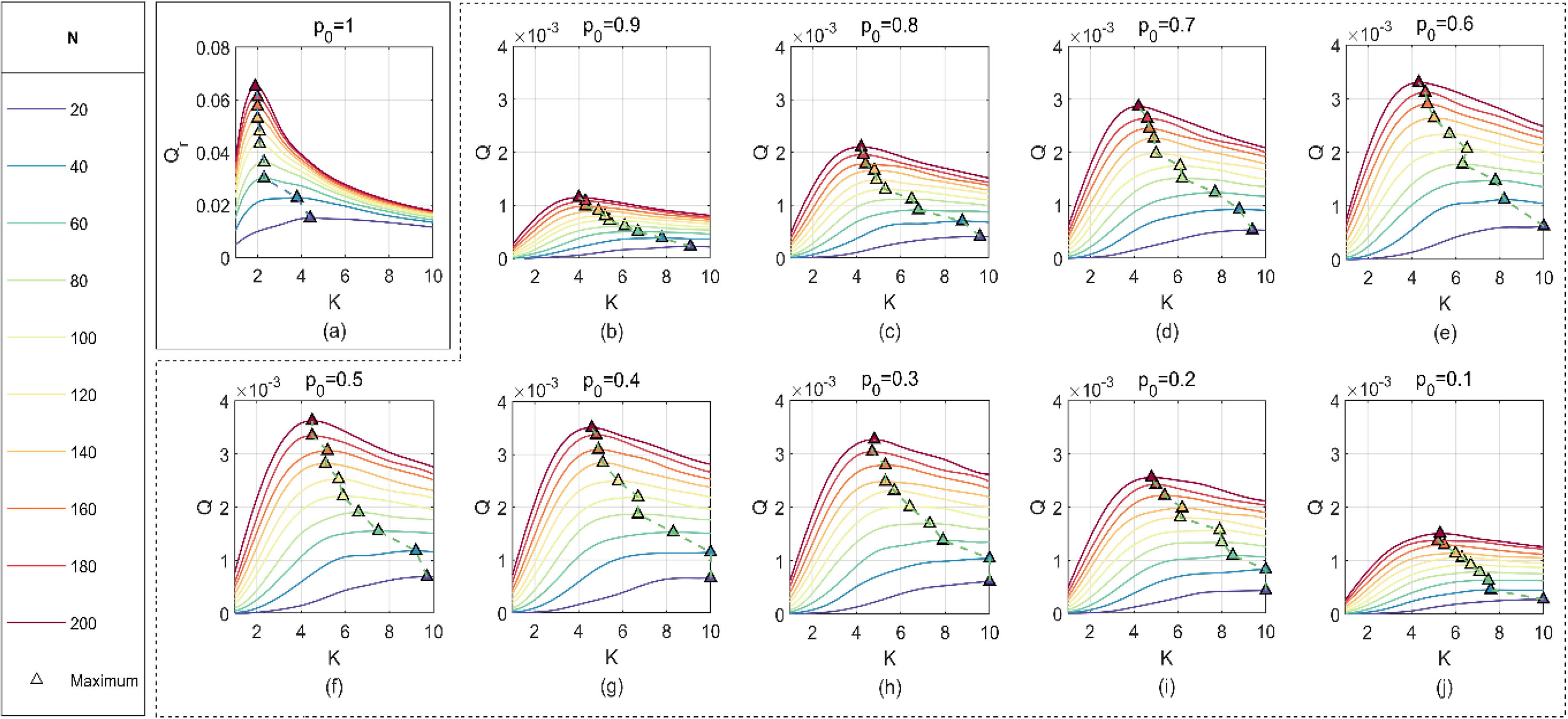
Figure 16 Influence of K on Q_r and Q with different values of N and p_0..

The least square algorithm (Wang P. et al., 2017; Zhou et al., 2019) is used to fit the points in Figure 16. While p₀ increases from 0.1 to 0.9, the optimum value of K can be estimated as follows:

$\begin{array}{ll}K=\{\begin{array}{l}-4.765N^{0.2115}+18.92,\hspace{0.17em}take\hspace{0.17em}Q\hspace{0.17em}as\hspace{0.17em}the\hspace{0.17em}standard\hspace{0.17em}133.2N^{-1.216}-1.657,\hspace{0.17em}take\hspace{0.17em}{Q}_r\hspace{0.17em}as\hspace{0.17em}the\hspace{0.17em}standard\hfill \end{array}& (26)\end{array}$

It can be seen from Figure 17 that the optimum value of K is more conservatively estimated, while Q_r is used as the evaluating criterion. It is worth noting that the optimum value of K tends to be 2 when N ≥ 60.

FIGURE 17

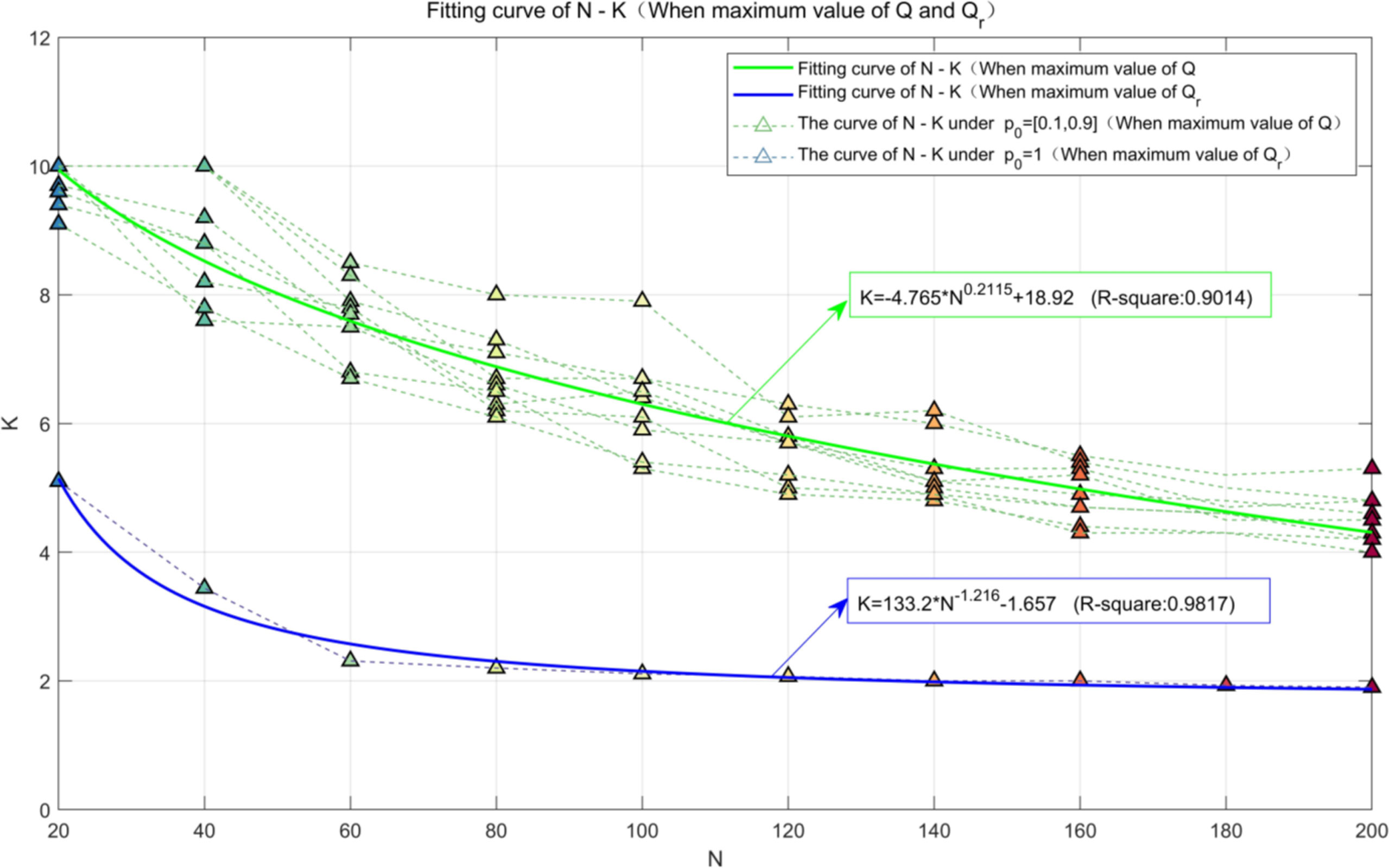
Figure 17 Influence of N on K when Q or Q_r is the maximum value.

When p₀ = 0.5 and W = 2, the performance indicators corresponding to the maximum value of Q are shown in Table 5. It can be seen from Table 5 that as N increases, both Δp and Δr increase while the optimum value of K decreases gradually.

TABLE 5

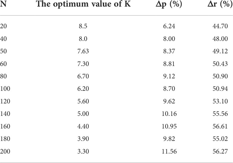
Table 5 Evaluation indicators (p₀ = 0.5, W = 2, and Q is the maximum value).

3) Influence of p₀ and N on Q

The relationship between p₀, N, and Q will affect the applicability of the CPS. In the actual picking process, p₀ and N are usually constant values, and the curves of Q varying with p₀ and N are shown in Figure 18.

FIGURE 18

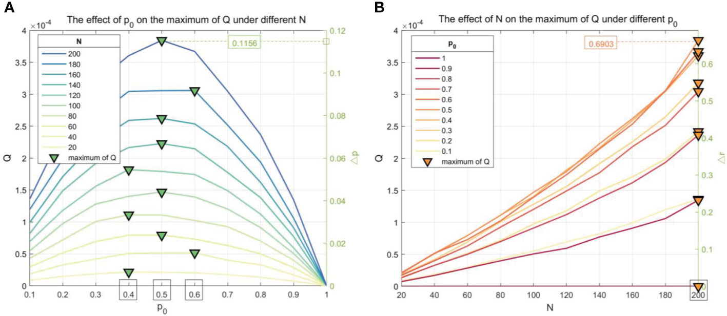
Figure 18 The curves of Q varying with p₀ and N. (A) The effect of p₀ on the maximum of Q under different N. (B) The effect of N on the maximum of Q under different p_0..

When N = [20, 200], it can be seen from the left vertical axis in Figure 18A that the curve of p₀-Q is approximately parabolic, and Q reaches the maximum value when p₀ is 0.5, which means that the CPS is superior to the SPS obviously when p₀ is closer to 0.5. The right vertical axis in Figure 18A shows that Δp increases from 0% to 11.56% with N increasing from 20 to 200. It can be seen from Figure 18B that the curve of N-Q increases monotonously, which means that the CPS is superior to the SPS if there are more buds. The right vertical axis in Figure 18B shows that Δr increases from 0% to 69.03% with N increasing from 20 to 200, which means less number of picking of the CPS.

Conclusion

A matrix mathematical model has been established for a picking box, and its parameters were fine-tuned. The CPS was innovatively put forward for picking the buds in a picking area. Compared with the SPS, it has the characteristics of higher picking efficiency, overall picking success rate, and shorter consumed time. The results of this study are as follows:

1) Fifty buds are randomly distributed in a picking area of 100 × 50 (cm²), and L and W are set as 6 and 2 cm, respectively. The experimental results of 100 random distributions show that compared to the SPS, the number of picking, the shortest picking path, and the average consumed time of the CPS were greatly reduced.

2) Picking results were analyzed according to L and W of a picking box, the single-point picking rate p₀, and the total number of buds N. The closer p₀ is to 0.5, the higher the yield per unit area Q of CPS. When p₀ = 0.5, the overall picking rate can increase from 0% to 11.56% with N increasing from 20 to 200.

3) Both L and W are closely related to the number of all buds in a peaking area N. Experimental results show that the optimal length-to-width ratio of a picking box can be calculated by K = -4.765N^0.2115 + 18.92, so the optimal sizes of the picking box can be calculated for picking areas with different distribution densities. While the picking efficiency is more emphasized, K = 133.2N^-1.216 – 1.657 is selected instead.

Experimental results show that the CPS greatly improved the overall picking rate and picking efficiency. In fact, to simplify the problem, the CPS abstracted the buds into some coordinate points and set a fixed single-point picking rate p₀, thus resulting in a few buds that cannot be covered by the picking box and difficulty ensuring the constant value of p₀ in actuality. Therefore, the follow-up study will solve the problems from three aspects: 1) Consider the sizes of buds while seeking the optimal coverage picking box set; 2) More factors that affect p₀ will be analyzed further; 3) The CPS will be further demonstrated, and the optimal sizes of a picking box will be designed more accurately.

Data availability statement

The raw data supporting the conclusions of this article will be made available by the authors, without undue reservation.

Author contributions

LX: Conceptualization, Investigation, Writing-original draft, Writing-review and editing. XC: Conceptualization, Investigation, Writing-original draft, Writing-review and editing. YC, YX and ZK: Methodology, Analysis, Suggestion. PH, HY and ZZ: Writing-review and editing, Analysis, Suggestion. ZL and LM: Writing-review and editing, Analysis, Suggestion. JD, ZW and BL: Writing-review and editing, Analysis, Suggestion. NY, YW and YZ: Validation, Resources, Supervision, Project administration, Writing-review and editing, Funding acquisition. All authors contributed to the article and approved the submitted version.

Funding

This study was funded by the Science and Technology Innovation Cultivation Project of Department of Science and Technology of Sichuan province (Grant No. 2021JDRC0091), the Key R & D project of Department of Science and Technology of Sichuan province (Grant No. 2020YFN0025).

Conflict of interest

The authors declare that the research was conducted in the absence of any commercial or financial relationships that could be construed as a potential conflict of interest.

Publisher’s note

All claims expressed in this article are solely those of the authors and do not necessarily represent those of their affiliated organizations, or those of the publisher, the editors and the reviewers. Any product that may be evaluated in this article, or claim that may be made by its manufacturer, is not guaranteed or endorsed by the publisher.

References

Cheein, F. A. A., Guivant, J. (2014). Slam-based incremental convex Hull processing approach for treetop volume estimation. Comput. Electron. Agric. 102, 19–30. doi: 10.1016/j.compag.2014.01.002

CrossRef Full Text | Google Scholar

Cheng, P., Yan, H., Han, Z. (2008). An algorithm for computing the minimum area bounding rectangle of an arbitrary polygon. J. Eng. Graph. 29 (1), 122–126. doi: 10.3969/j.issn.1003-0158.2008.01.022

CrossRef Full Text | Google Scholar

Chen, M., Tang, Y., Zou, X., Huang, K., Huang, Z., Zhou, H., et al. (2020). Three-dimensional perception of orchard banana central stock enhanced by adaptive multi-vision technology. Comput. Electron. Agric. 174, 105508. doi: 10.1016/j.compag.2020.105508

CrossRef Full Text | Google Scholar

Chen, M., Tang, Y., Zou, X., Huang, Z., Zhou, H., Chen, S. (2021). 3D global mapping of large-scale unstructured orchard integrating eye-in-hand stereo vision and SLAM. Comput. Electron. Agric. 187, 106237. doi: 10.1016/j.compag.2021.106237

CrossRef Full Text | Google Scholar

Deng, Y., Zhu, W., Li, H., Zheng, Y. (2018). Multi-type ant system algorithm for the time dependent vehicle routing problem with time windows. J. Syst. Eng. Electron. 29 (3), 625–638. doi: 10.21629/jsee.2018.03.20

CrossRef Full Text | Google Scholar

Du, Z., Zhe, H., Wang, S. (2018). Simulation and experiment of reciprocating cutter kinematic of portable tea picking machine. Trans. Chin. Soc. Agric. Machinery 49 (S1), 221–226. doi: 10.6041/j.issn.1000-1298.2018.S0.029

CrossRef Full Text | Google Scholar

Gao, Y., Cheng, Y., Wang, X. (2015). A quick convex Hull building algorithm based on grid and binary tree. Chin. J. Electron. 24 (2), 317–320. doi: 10.1049/cje.2015.04.015

CrossRef Full Text | Google Scholar

Han, Y., Xiao, H., Qin, G., Song, Z., Ding, W., Mei, S. (2014). Studies on develop situations of tea-leaf picker both at home and abroad. Chin. Agric. Mech. 35 (2), 20–24. doi: 10.13733/j.jcam.issn.2095-5553.2014.02.006

CrossRef Full Text | Google Scholar

Jiang, Z., Zhou, M., Tong, J., Jiang, H., Yang, Y., Wang, A., et al. (2015). Comparing an ant colony algorithm with a genetic algorithm for replugging tour planning of seedling transplanter. Comput. Electron. Agric. 113, 225–233. doi: 10.1016/j.compag.2015.02.011

CrossRef Full Text | Google Scholar

Lin, G., Zhu, L., Li, J., Zou, X., Tang, Y. (2020). Collision-free path planning for a guava-harvesting robot based on recurrent deep reinforcement learning. Computers and Electronics in Agriculture 188, 106350. doi: 10.1016/j.compag.2021.106350

CrossRef Full Text | Google Scholar

Li, J., Tang, Y., Zou, X., Lin, G., Wang, H. (2020). Detection of fruit-bearing branches and localization of litchi clusters for vision-based harvesting robots. IEEE Access 8, 117746–117758. doi: 10.1109/ACCESS.2020.3005386

CrossRef Full Text | Google Scholar

Lu, X., Li, H., Xu, L., Qin, G., Zhao, Y. (2015). The improve design of tea picking robot with two arms. J. Agric. Mech. Res. 37 (2), 101–106. doi: 10.13427/j.cnki.njyi.2015.02.025

CrossRef Full Text | Google Scholar

Park, J., Lim, H. (2014). Bounding box extraction from spherical hologram of elementary object to synthesize hologram of arbitrary three-dimensional scene with occlusion consideration (invited paper). Chin. Opt. Lett. 12 (6), 90–94. doi: 10.3788/COL201412.060019

CrossRef Full Text | Google Scholar

Qin, G., Zhao, Y., Xiao, H., Jin, Y., Xu, L., Chen, Y. (2014). 4CZ―12 intelligent tea harvest robot design and field experiment. J. Chin. Agric. Mech. 35 (1), 152–156,169. doi: 10.3969/j.issn.2095-5553.2014.01.035

CrossRef Full Text | Google Scholar

Song, H., He, D., Pan, J. (2012). Recognition and localization methods of occluded apples based on convex hull theory. Trans. Chin. Soc. Agric. Eng. 28 (22), 174–180. doi: 10.3969/j.issn.1002-6819.2012.22.025

CrossRef Full Text | Google Scholar

Tang, Y., Chen, M., Wang, C., Luo, L., Li, J., Lian, G., et al. (2020). Recognition and localization methods for vision-based fruit picking robots: A review Front Plant Sci 11, 510. doi: 10.3389/fpls.2020.00510

PubMed Abstract | CrossRef Full Text | Google Scholar

Tang, Y., Han, W., Hu, A. (2016). Design and experiment of intelligentized tea-plucking machine for human riding based on machine vision. Trans. Chin. Soc. Agric. Machinery 47 (7), 15–20. doi: 10.6041/j.issn.1000-1298.2016.07.003

CrossRef Full Text | Google Scholar

Tang, L., Hou, W., Liu, L., Cao, W., Zhu, Y. (2018). Collision detection of virtual plant based on bounding volume hierarchy:A case study on virtual wheat. J. Integr. Agric. 17 (2), 306–314. doi: 10.1016/S2095-3119(17)61769-6

CrossRef Full Text | Google Scholar

Tong, J., Wu, C., Jiang, H., Yu, Y., Rao, X. (2017). Optimizing the path of seedling low-density transplanting by using greedy genetic algorithm. Comput. Electron. Agric. 142, 356–368. doi: 10.1016/j.compag.2017.09.017

CrossRef Full Text | Google Scholar

Wang, H., Gao, G., Xia, Q., Li, L., Ren, H. (2018). Establishment and verification on static equivalent model of end load posture of continuum picking manipulator. Trans. Chin. Soc. Agric. Eng. 34 (05), 23–31. doi: 10.11975/j.issn.1002-6819.2018.05.004

CrossRef Full Text | Google Scholar

Wang, C., Tang, Y., Zou, X., Luo, L., Chen, X. (2017). Recognition and matching of clustered mature litchi fruits using binocular charge-coupled device (CCD) color cameras. Sensors 17, 11, 2564. doi: 10.3390/s17112564

CrossRef Full Text | Google Scholar

Wang, L., Xia, X., Cao, J., Liu, X., Liu, J. (2018). Improved ant colony-genetic algorithm for information transmission path optimization in remanufacturing service system. Chin. J. Mech. Eng. 31 (6), 106–117. doi: 10.1186/s10033-018-0311-9

CrossRef Full Text | Google Scholar

Wang, P., Yu, Q., Hu, Y., Miao, C. (2017). Online detection of broken rotor bar fault in induction motors by combining estimation of signal parameters Via Min-norm algorithm and least square method. Chin. J. Mech. Eng. 30 (6), 1285–1295. doi: 10.1007/s10033-017-0185-2

CrossRef Full Text | Google Scholar

Wang, P., Zhang, T., Xiao, J. (2020). Application research of ant colony cellular optimization algorithm in population evacuation path planning. Acta Phys. Sin. 69 (08), 240–248. doi: 10.7498/aps.69.20191774

CrossRef Full Text | Google Scholar

Wei, X., Han, J. (2016). Smallest enclosing rectangle planning for spatial target distribution on the basis of boolean search. J. South China Univ. Technol. (Nat. Sci. Ed.) 44 (5), 144–150. doi: 10.3969/j.issn.1000-565X.2016.05.022

CrossRef Full Text | Google Scholar

Wen, G., Zhang, Q., Wang, H., Tian, Q., Tao, Y. (2017). An ant colony algorithm based on cross-layer design for routing and wavelength assignment in optical satellite networks. China Commun. 14 (8), 63–75. doi: 10.1109/CC.2017.8014348

CrossRef Full Text | Google Scholar

Yan, F., Liu, Y., Xiao, J. (2013). Path planning in complex 3d environments using a probabilistic roadmap method. Int. J. Autom. Comput. 10 (6), 525–533. doi: 10.1007/s11633-013-0750-9

CrossRef Full Text | Google Scholar

Yuan, Y., Zheng, X., Lin, W. (2017). Path planning of picking robot for famous tea. J. Anhui Agric. Univ. 44 (3), 530–535. doi: 10.13610/j.cnki.1672-352x.20170524.030

CrossRef Full Text | Google Scholar

Zhang, H., Chen, Y., Wang, W., Zhang, G. (2014). Positioning method for tea picking using active computer vision. tea in fujian. Trans. Chin. Soc. Agric. Machinery 45 (9), 61–65, 78. doi: 10.6041/j.issn.1000-1298.2014.09.010

CrossRef Full Text | Google Scholar

Zhang, C., Xu, H., Jiang, H. (2018). Adaptive block greedy algorithms for receiving multi-narrowband signal in compressive sensing radar reconnaissance receiver. J. Syst. Eng. Electron. 29 (6), 1158–1169. doi: 10.21629/jsee.2018.06.05

CrossRef Full Text | Google Scholar

Zhang, X., Zhang, W., Zhou, R., Xiang, Z. (2019). Anomaly detection method based on one-class random forest with applications. J. Xi'an Jiaotong Univ. 54 (02), 1–8+157. doi: 10.7652/xjtuxb202002001

CrossRef Full Text | Google Scholar

Zhao, N., Ye, S., Li, K., Chen, S. (2017). Effective iterated greedy algorithm for flow-shop scheduling problems with time lags. Chin. J. Mech. Eng. 30 (3), 652–662. doi: 10.1007/s10033-017-0108-2

CrossRef Full Text | Google Scholar

Zhou, Z., Morel, J., Parsons, D., Kucheryavskiy, S. V., Gustavsson, A. M. (2019). Estimation of yield and quality of legume and grass mixtures using partial least squares and support vector machine analysis of spectral data. Comput. Electron. Agric. 162, 246–253. doi: 10.1016/j.compag.2019.03.038

CrossRef Full Text | Google Scholar