Estimating the full-period rice leaf area index using CNN-LSTM-Attention and multispectral images from unmanned aerial vehicles

Introduction: Leaf area index (LAI) of rice is a crucial parameter for assessing the growth conditions and predicting yields. However, traditional measurement methods are inefficient and insufficient for large-scale monitoring.

Methods: This study proposes a CNN-LSTM-Attention (CLA) model that integrates convolutional neural networks (CNN), long short-term memory (LSTM), and a self-attention mechanism, aiming to achieve high-precision estimation of rice LAI across all growth stages based on the unmanned aerial vehicle (UAV) multispectral imagery and deep learning techniques. The estimation performance of vegetation indices (VIs), machine learning methods (SVR, RFR, PLSR, XGBoost), and deep learning models (DNN, CNN, LSTM) were comparatively analyzed.

Results and discussion: The results show that the CLA model outperforms other approaches in estimating rice LAI throughout the entire growing period, achieving a coefficient of determination (R²) of 0.92 and a relative root mean square error (RRMSE) below 9%, significantly better than linear regression and machine learning methods. Moreover, the CLA model maintains high stability and accuracy across different LAI ranges, with notably reduced errors for low LAI values (one to three), effectively mitigating the influence of soil background. This research offers an efficient and accurate technological approach for rice growth monitoring and holds significant implications for precision agricultural management.

1 Introduction

Rice is one of the world’s most important staple crops, together with maize and wheat, providing approximately 30% of caloric intake in 94 developing countries (Wang et al., 2025). Consequently, effectively monitoring rice growth and health has become an urgent and significant issue. The leaf area index (LAI), defined as the total one-sided leaf surface area per unit ground area, is tightly linked to diverse vegetation parameters like pigment content, growth density, and disease and pest levels (Chen and Black, 1992; Yan et al., 2019). Furthermore, LAI acts as a crucial proxy of crop photosynthesis and growth status and plays an essential role in yield prediction (Roosjen et al., 2018). As a critical parameter for evaluating canopy photosynthetic capacity, LAI significantly affects crop productivity throughout the growing season (Zhang et al., 2021). Dynamic monitoring of LAI provides valuable insights into the crop’s response to environmental changes and allows for more accurate yield evaluation (Jay et al., 2017).

Currently, LAI is commonly measured by lossy sampling and non-contact measurements. The first offers relatively accurate results but are labor-intensive and inefficient, rendering them impractical for large-scale automated monitoring (Yuan et al., 2017). Indirect methods, often employing optical instruments, are also limited by low efficiency and inadequate capacity for rapid, large-scale assessment (Bhadra et al., 2024). Satellite remote sensing enables large-area data acquisition, but its low spatial and temporal resolution makes it unsuitable for precision agriculture (Fang et al., 2019). In contrast, low-altitude remote sensing represented by unmanned aerial vehicle (UAV) has come to the fore as a superior alternative due to its ability to collect data flexibly and at high resolution over large areas. In the past few years, UAV remote sensing has played an increasingly significant role in agricultural surveillance because of its excellent spatial and temporal details and operational flexibility (Yue et al., 2023, 2023). Multispectral cameras mounted on UAVs can acquire high-resolution (centimeter-level) data across multiple spectral bands (from visible to near-infrared), offering an effective balance between cost and usability (Deng et al., 2018). Therefore, this study adopts UAV multispectral imagery as the primary data source.

Canopy reflectance, captured by remote sensing sensors deployed on various platforms from ground to satellite, is primarily influenced by vegetation absorption and scattering (Yu et al., 2024), both of which are strongly correlated with crop LAI (Zou et al., 2024). By integrating reflectance across multiple bands into vegetation indices (VIs) (Jay et al., 2017; Kross et al., 2015), and applying multivariate regression and machine learning techniques using multispectral or hyperspectral data, effective methods have been developed for extracting spectral features essential to LAI estimation (Zou et al., 2024). Remote sensing-based inversion methods offer a new and efficient approach for large-scale, rapid, and accurate LAI assessment, allowing better representation of its spatial distribution and temporal dynamics (Liang et al., 2015; Yang et al., 2017). These methods also enhance our understanding of LAI variation, contributing to improved vegetation ecosystem management (Li et al., 2022). In addition to these methods, physically-based inversion approaches have also been employed for LAI retrieval. For example, high-precision models have been constructed for rice LAI estimation using the PROSAIL model combined with Bayesian networks (Xu et al., 2019). Yue et al. proposed a hybrid LAI estimation approach for wheat, maize, potato, rice, and soybean using deep learning and hyperspectral data integrated with radiative transfer models, achieving significantly higher accuracy than traditional statistical regression techniques (Yue et al., 2024). Although physically-based models offer clear interpretability, they require numerous input parameters and involve complex processes, often leading to ill-posed inversion problems, thus limiting their practical applicability.

Numerous studies have demonstrated the effectiveness of VI-based remote sensing models in estimating the LAI of field crops (Liang et al., 2020; Ma et al., 2022). Although multispectral images are relatively cost-effective, their limited spectral bands can lead to issues such as spectral confusion (same spectrum, different objects or vice versa). Texture features, another important source of remote sensing information, reflect spatial variation characteristics in the imagery. Many researchers have combined spectral and texture features to estimate LAI for different crops, showing that incorporating texture information can improve LAI monitoring accuracy (Li et al., 2019; Zhuang et al., 2024; Zhang et al., 2022). However, the role and optimal scale of various texture types in estimating canopy LAI for crops like wheat and maize remain unclear, and their underlying mechanisms are difficult to interpret. Furthermore, most prior studies have focused on a single or a few growth stages, with limited research covering the entire crop growth cycle.

There are two main challenges that hinder the practical application of remote sensing-based LAI estimation models. First, during the early stages of crop growth, soil background interference leads to inaccurate canopy information (Yue et al., 2024). In rice, low LAI values during the seedling stage result in large proportions of exposed soil, with leaves primarily growing horizontally. Given the distinct spectral characteristics between soil and rice leaves, direct use of canopy spectra can compromise estimation accuracy (Jay et al., 2017). Therefore, removing soil background effects is essential for improving LAI estimation. Several background removal methods have been proposed and shown effective for crop monitoring (Liu et al., 2023; Darvishzadeh et al., 2008). However, their performance significantly declines in low-resolution images. For example, imagery captured at high UAV altitudes using multispectral or hyperspectral cameras often lacks sufficient resolution for soil-background separation. Second, during the mid-to-late stages of crop growth, vegetation canopy becomes denser with vertically growing leaves, leading to VIs saturation and reduced LAI estimation accuracy and model generalizability (Li and Liang, 2023). To address this, fusing multimodal remote sensing data (e.g., thermal infrared, hyperspectral, LiDAR) has been shown to mitigate indices saturation (Zhang et al., 2024, 2023). Nonetheless, the data acquisition and processing costs remain high, limiting widespread application.

With the rapid development of artificial intelligence, machine learning (ML) and deep learning (DL) techniques have emerged as powerful tools for estimating crop LAI (Li et al., 2025). Traditional ML algorithms, including partial least squares regression (PLSR), artificial neural networks (ANN) (Liang et al., 2020), Gaussian process regression (GPR) (Sinha et al., 2020), Bayesian algorithms, support vector regression (SVR), and random forest regression (RFR) (Li et al., 2019; Yue et al., 2018), have demonstrated effectiveness in crop LAI prediction, particularly in scenarios with limited training data. Among these, ANN, a computational model inspired by biological neural networks, has outperformed empirical methods in estimating biophysical parameters due to its superior nonlinear modeling capability (Danson et al., 2003). For instance, a multimodal deep neural network (DNN) framework achieved higher accuracy than SVR, RFR, and PLSR in LAI estimation across different growth stages (Liu et al., 2021). Similarly, an improved convolutional neural network (CNN) accurately estimated maize LAI at critical developmental phases, including jointing, small trumpet, and large trumpet stages (Yang et al., 2025).

Despite these advancements, conventional ML methods face limitations in handling large-scale spatiotemporal data due to their reliance on manual feature engineering and weak temporal modeling capacity. Deep learning, particularly recurrent neural networks (RNNs), has addressed these challenges by automatically extracting hierarchical features from raw data. Long short-term memory (LSTM), a specialized RNN variant, has shown exceptional performance in time-series LAI estimation by capturing long-range dependencies in multitemporal remote sensing data (Liu et al., 2025). However, existing approaches often neglect the dynamic importance of different growth stages, leading to suboptimal performance in full-season LAI estimation. To overcome these limitations, we propose an integrated CNN-LSTM-Attention framework for accurate and adaptive rice LAI estimation across the entire growth cycle. This model synergistically combines: (1) CNN extracts high-level spatial features from multispectral imagery, capturing localized crop canopy structures; (2) LSTM models temporal dependencies in LAI dynamics, accounting for cumulative environmental effects (e.g., temperature, precipitation) on crop growth; and (3) attention mechanism dynamically weights critical growth stages (e.g., tillering, heading) to enhance model interpretability and prediction robustness.

Against the above presentation, this study integrates CNN, LSTM, and a self-attention mechanism to effectively capture the spatial and temporal features of rice canopy spectral data, thereby constructing an accurate LAI estimation model across the entire growing season. The proposed approach is also compared with traditional linear regression and several commonly used machine learning methods. The main objectives and contributions of this study are (1) to develop a high-precision LAI estimation model by proposing a CLA model that combines CNN, LSTM, and self-attention mechanism, aiming to realize high-precision estimation of rice LAI during the whole growing season; (2) to evaluate the different methods’ performance by comparing and analyzing the performance of VIs, traditional machine learning methods (SVR, RFR, PLSR, and XGBoost), and deep learning models (DNN, CNN, LSTM) in LAI estimation; and (3) to solve the challenges of practical applications by addressing the problems of soil background disturbance in the early stage of rice growth and the saturating of vegetation indices in the middle and late stages, proposing effective solutions to improve the stability and accuracy of the model in different LAI ranges.

2 Materials and Methods

2.1 Experimental design

The study utilized 30 rice varieties, with each variety planted in a separate plot, totaling 30 experimental plots under normal field management conditions in Xinyang city, Henan province. All plots received consistent cultivation practices including irrigation, fertilization, and pest control to ensure uniform growing conditions across the study area (as shown in Figure 1). Rice seedlings were sown on May 10, 2024, and transplanted on June 12 at a uniform spacing of 0.25 m × 0.25 m, with a planting density of 25 plants/m².

Figure 1

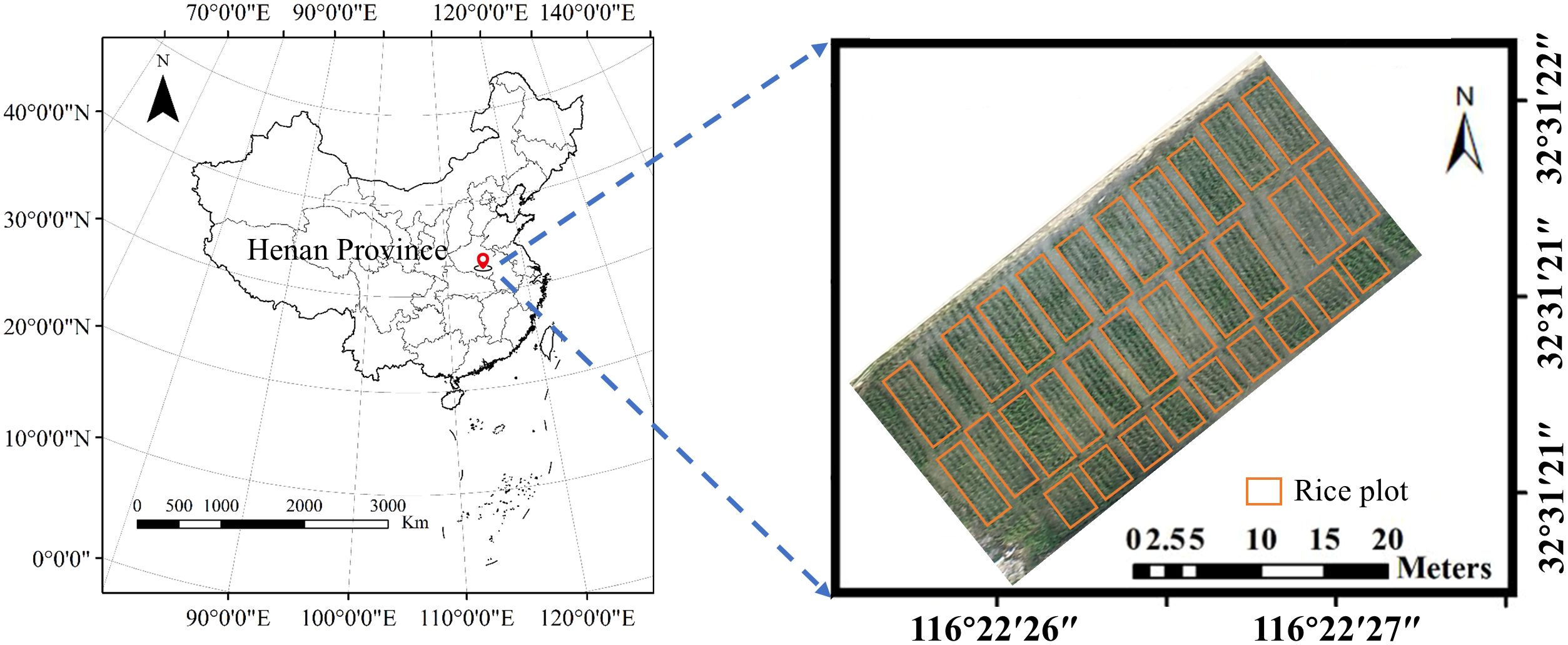
Figure 1. Experimental design and plots distribution.

2.2 LAI data acquisition

The rice LAI data (unit: m²/m²) were measured using a LI-COR LAI-2200C Plant Canopy Analyzer (LI-COR Biosciences, USA). Prior to each measurement, the LAI measuring instrument was recalibrated to guarantee reliability, and care was taken to avoid operation under direct sunlight. Measurements were conducted between 9:00–10:00 a.m. and 3:00–5:00 p.m. (local time). Ten replicate observations were carried out in each plot to ensure coverage of the regional spatial diversity of the rice population. Field measurements were synchronized with UAV image acquisition, covering key rice growth stages: tillering, jointing, booting, heading, grain filling, milky, and maturity stages, on the following dates: June 30 (S1), July 10 (S2), July 19 (S3), July 25 (S4), August 5 (S5), August 14 (S6), August 28 (S7), September 5 (S8), and September 12 (S9), totaling 9 time points. The approximate interval between these data acquisition dates is one week.

2.3 UAV multispectral image acquisition and processing

In this study, an octocopter UAV was utilized to carry a multispectral camera (RedEdge-P), which was composed of 5 individual miniature cameras. Each camera was equipped with different filter sizes to obtain the radiation information in the desired wavelength band, and the corresponding center wavelengths and band widths of the 5 cameras are shown in Table 1. The selected bands span the visible to near-infrared regions (Kimes et al., 1981), including red-edge bands known for their utility in crop surveillance (Schlemmer et al., 2013; Clevers and Gitelson, 2013). Flights were executed between 10:00 a.m. and 2:00 p.m. under clear sky and no wind conditions, with a flight altitude of 40 m. All UAV flights were conducted under strictly controlled environmental conditions to ensure data quality. Single UAV flights were limited to three minutes to ensure that light variations were minimal. The UAV shootings produced images with a resolution of 1456×1088 pixels and a ground sampling distance of 2.6 cm/pixel.

Table 1

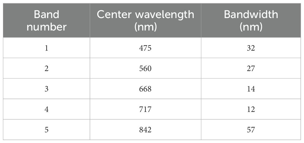
Table 1. Bands information of multispectral camera.

Data processing is a critical step in UAV-based multispectral data analysis, as raw images captured by the RedEdge-P camera require correction and calibration before further use. The initial pixel values lack physical meaning and often contain geometric and radiometric distortions. The processing workflow includes geometric correction, image stitching, and radiometric calibration, all performed using Pix4D Mapper (Pix4D SA, Prilly, Switzerland). First, the raw multispectral images (in .tiff format) were imported into Pix4D for automatic geometric correction and image stitching. The software utilized the embedded GPS/IMU data from the M350 drone and ground control points to align and orthorectify the images, minimizing distortions caused by terrain variations and camera tilt. After processing, the software generated a high-resolution orthomosaic and a digital surface model (DSM). A comparison between pre- and post-geometric correction is illustrated in Figure 2. Before correction, the RGB composite image exhibited noticeable pixel misalignment, with significant distortions and shape deformations that sometimes rendered objects unrecognizable. After geometric correction, the misalignment and distortion were effectively eliminated, resulting in sharper object boundaries and improved overall image clarity. Radiometric calibration was then applied to convert raw digital numbers into reflectance values. This process involved using reference tarps with known reflectance to derive the reflectance of other targets in the scene. Before each flight, three calibration tarps made of polyester fabric with known reflectance values (0.10, 0.30, 0.50) were placed on flat ground for radiometric calibration. The piecewise empirical line (PEL) method was used for calibration (Luo et al., 2022). As shown in Figure 2, a comparison of UAV multispectral images before and after radiometric calibration reveals significant improvements in image quality. Prior to calibration, the RGB composite image appears visibly darker, with low contrast between rice plants and other ground objects. After radiometric calibration, the RGB composite image exhibits enhanced brightness, significantly improving the distinguishability of rice canopies from surrounding features. Additionally, the soil background, field ridges, and pathways become more clearly delineated, resulting in sharper details across the entire image.

Figure 2

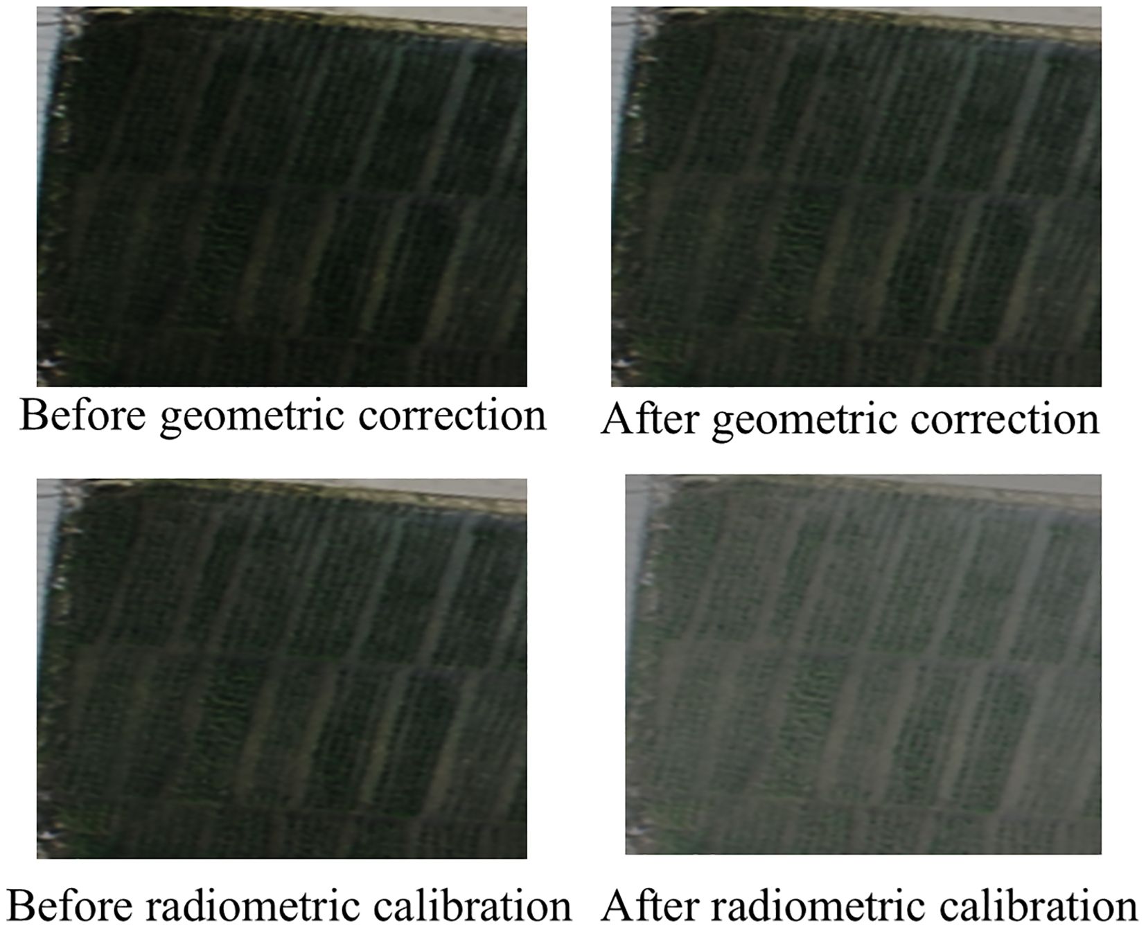
Figure 2. Comparison of multispectral images before and after preprocessing.

2.4 Selection and calculation of vegetation indices

Vegetation indices, computed from combinations of spectral bands, are widely used to enhance crop canopy signals, which have been proved to be effective in LAI estimation. Indices such as NDVI, SAVI, EVI2 have showed excellent results in LAI inversion (Han et al., 2021). Lately, red-edge-based indices such as NDRE (Gitelson and Merzlyak, 1994) and CI_{red edge} (Gitelson et al., 2003) have gained attention for their superior performance, particularly when there is a thick cover (Delegido et al., 2013; Deng et al., 2018; Wang et al., 2022). Based on the above prior knowledge, fifteen vegetation indices as shown in Table 2 were considered and selected for this study. Since these VIs have been demonstrated to exhibit superior performance in crop growth monitoring, after the importance ranking analysis, we incorporated several important VIs for rice LAI estimation as input variables during model construction.

Table 2

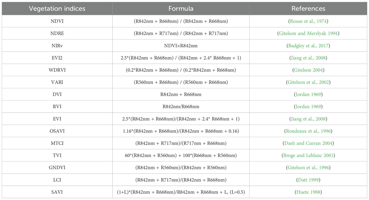
Table 2. The vegetation indices used in this study and their calculations.

2.5 Deep learning methods

2.5.1 CNN

CNNs are primarily used to extract spatial features from sequential or structured data. By applying convolutional kernels that slide across the input data, CNNs are capable of quickly identifying local layouts, like edges in pictures or certain waveforms in time-series data. In sequence modeling, CNNs are capable of capturing local dependencies within the input by focusing on adjacent feature relationships (Du et al., 2025). The convolution operation is typically followed by pooling layers, which reduce the spatial dimensions of the feature maps and help decrease computational complexity while preserving the most salient features. A standard CNN design was made up of five essential elements: input layers, convolutional layers, pooling layers, fully connected layers, and an output layer, as illustrated in Figure 3.

Figure 3

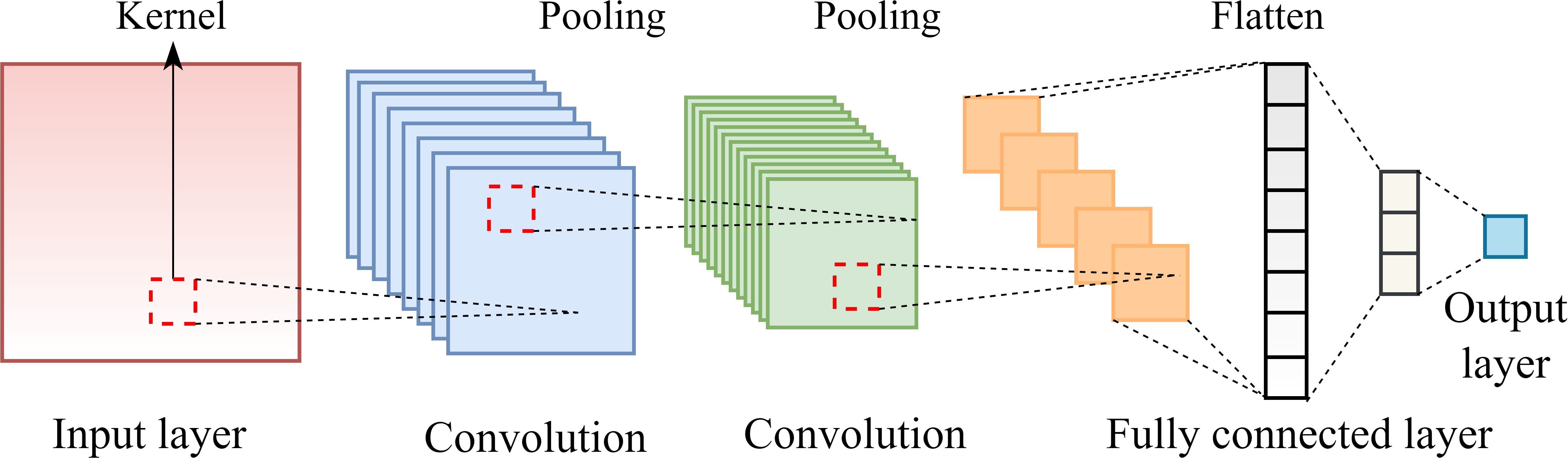
Figure 3. CNN model structure.

The input layer is responsible for receiving and pre-processing raw data. The convolutional layers usually contain multiple convolutional kernels of varying sizes, each responsible for learning specific patterns from the input. These layers are designed to extract significant information from the original data. Pooling layers perform downsampling on the outputs of convolutional layers, reducing feature dimensionality and network parameters while retaining essential information. The fully connected layers transform the three-dimensional feature maps produced by the pooling layers into a one-dimensional vector, which is then passed to subsequent layers (the output layers).

2.5.2 LSTM

The LSTM is an advanced network of the RNN, which is specialized in processing the temporal dependency in sequence data. It is capable of addressing the disappearance of the gradient problem that occurs when RNN learns sequences of too long duration, and may avoid the long-term dependency problem (Guo et al., 2024). Extensive studies have demonstrated the effectiveness of LSTM networks in processing various types of sequential data, including time-series signals, textual data, speech, and video (Murugesan et al., 2022). The primary breakthrough of LSTM depends on the connection of cell states, allowing for selective information retention and forgetting through three specialized gating mechanisms: the input gate, the forget gate, and the output gate. They regulate the flow of information, allowing the network to preserve related features and discarding the unrelated. The architecture of the LSTM network is illustrated in Figure 4. Bidirectional LSTM (BiLSTM) networks (Dhaka and Nagpal, 2023) were not considered due to considerations of temporal dependency directionality (future LAI values are primarily influenced by past and present conditions), computational efficiency (BiLSTM processes data in both forward and backward directions, doubling the parameters and training time compared to LSTM), avoidance of overfitting risks, and physical interpretability (crop growth follows unidirectional physiological processes).

Figure 4

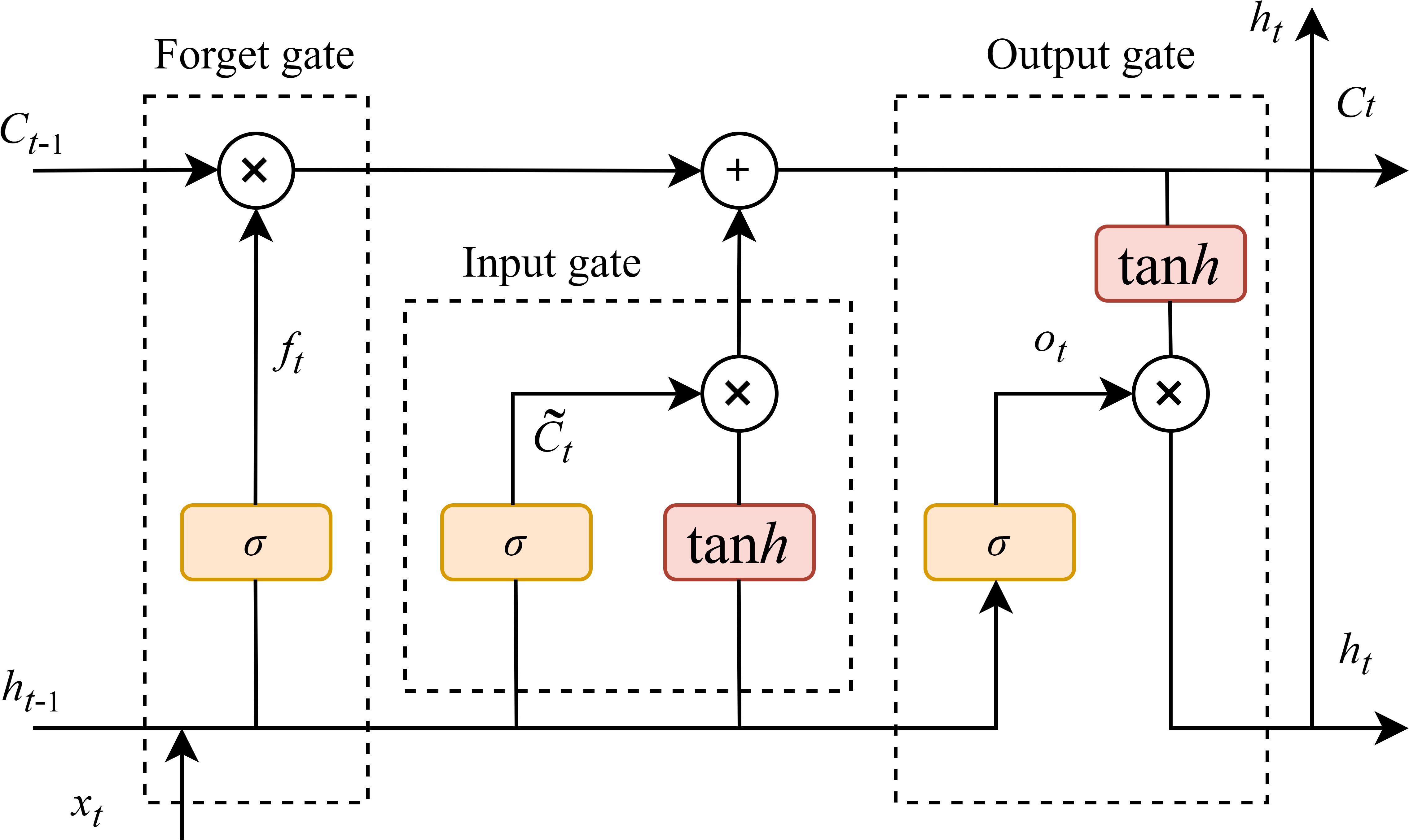
Figure 4. LSTM model structure(x_t is the model input, the hidden state at the previous time is h_t–1, the memory unit state at the previous time is C_t–1, the hidden state at the current time is h_t, and the memory unit state at the current time is C_t).

2.5.3 Attention mechanism

The self-attention mechanism is employed to compute the dependencies between different time steps within an input sequence. By calculating attention weights that reflect the relevance of each time step to every other time step, the model is able to perform a weighted aggregation of information across the entire sequence. This allows the model to dynamically focus on the most informative parts of the sequence while reducing the influence of less relevant components (Choi et al., 2018).

Attention mechanisms are categorized into hard and soft ones. The hard one operates as a stochastic process, attending to only one specific position at a time, typically represented using a one-hot vector. However, due to its discontinuous nature, it is not well-suited for time-series prediction tasks. In contrast, soft attention considers all positions simultaneously and assigns a learnable attention weight to each feature. This continuous and differentiable formulation makes it more appropriate for sequence modeling and prediction tasks. The following is a general expression (Equation 1) for the attention mechanism’s calculating:

$\begin{array}{ll}\begin{array}{c}{h}^{*}={\displaystyle \sum _{i=1}^k{\alpha }_i{h}_i}\end{array}& (1)\end{array}$

where h_iis the input data and h* is the final result. Self-attention is to calculate the weight α. We chose the additive self-attention to calculate the weight, and the Equations 2, 3 is as follows:

$\begin{array}{ll}\begin{array}{c}\alpha (s_{t-1,} h_j)=v_{\alpha }^{T}tanh(U_{\alpha }{h}_i+W_{\alpha }{s}_{t-1})\end{array}& (2)\end{array}$

where $W_{\alpha },U_{\alpha },v_{\alpha }$ is the weight matrix.

$\begin{array}{ll}\begin{array}{c}{\alpha }_{t,j}=\frac{\exp (\alpha (s_{t-1,} h_j))}{{\sum }_{j=1}^T\exp (\alpha (s_{t-1,} h_j))}\end{array}& (3)\end{array}$

where s_t-1 is the hidden state of t–1, a_t,_j is the weight of parameter j in time t.

2.5.4 CNN-LSTM-Attention

The CNN-LSTM-Attention (CLA) network is a hybrid architecture that integrates CNN, LSTM networks, and the attention mechanism. This model is specifically designed to capture both local spatial features and long-range temporal dependencies in sequential data, while dynamically focusing on the most informative time steps through the attention mechanism. The data processing flow of the CLA model consists of five main steps: 1). The input time series is reshaped into a matrix format compatible with neural network processing. 2). This matrix is fed into a CNN for local feature extraction and dimensionality reduction. 3). The extracted feature sequence is then passed to the LSTM network to model temporal dependencies. 4). An attention mechanism is applied to the LSTM output to compute a weighted average, allowing the model to emphasize important time steps. 5). Finally, a fully connected layer is used to generate the prediction output. The overall architecture of the CLA model is illustrated in Figure 5.

Figure 5

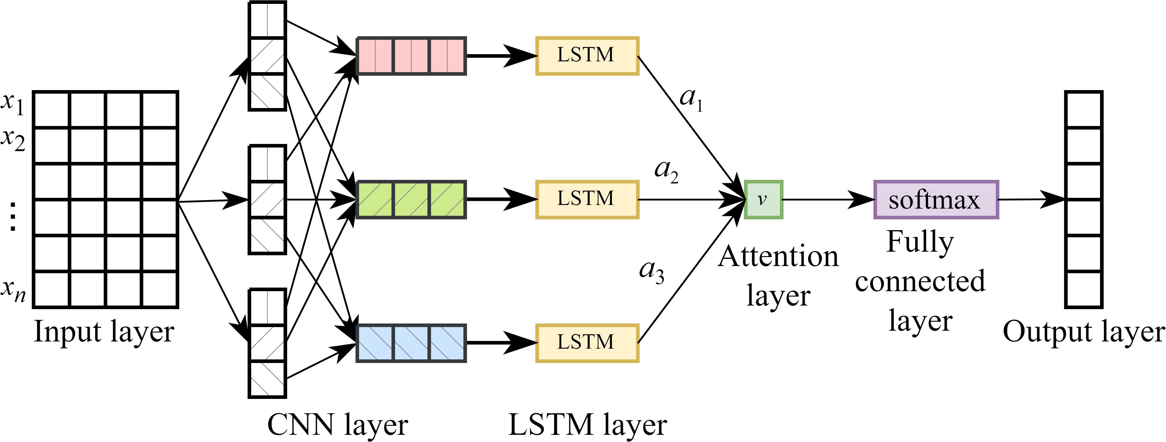
Figure 5. CLA model structure.

As shown in Figure 6, to address the generalization issue between the hidden states and output layer in LSTM networks, an attention mechanism is introduced between the hidden layer and the output layer. In the figure, x₁, x₂, …, x_n denote the input sequence at a given time step, while h₁, h₂, …, h_t represent the corresponding hidden states of the LSTM. By incorporating an attention mechanism after the hidden layer, attention weights α₁, α₂, …, α_t are computed for each hidden state. These weights are then used to perform a weighted average to obtain the context vector v, which is subsequently passed to a Softmax layer. The final output y is generated via a fully connected computation based on v.

Figure 6

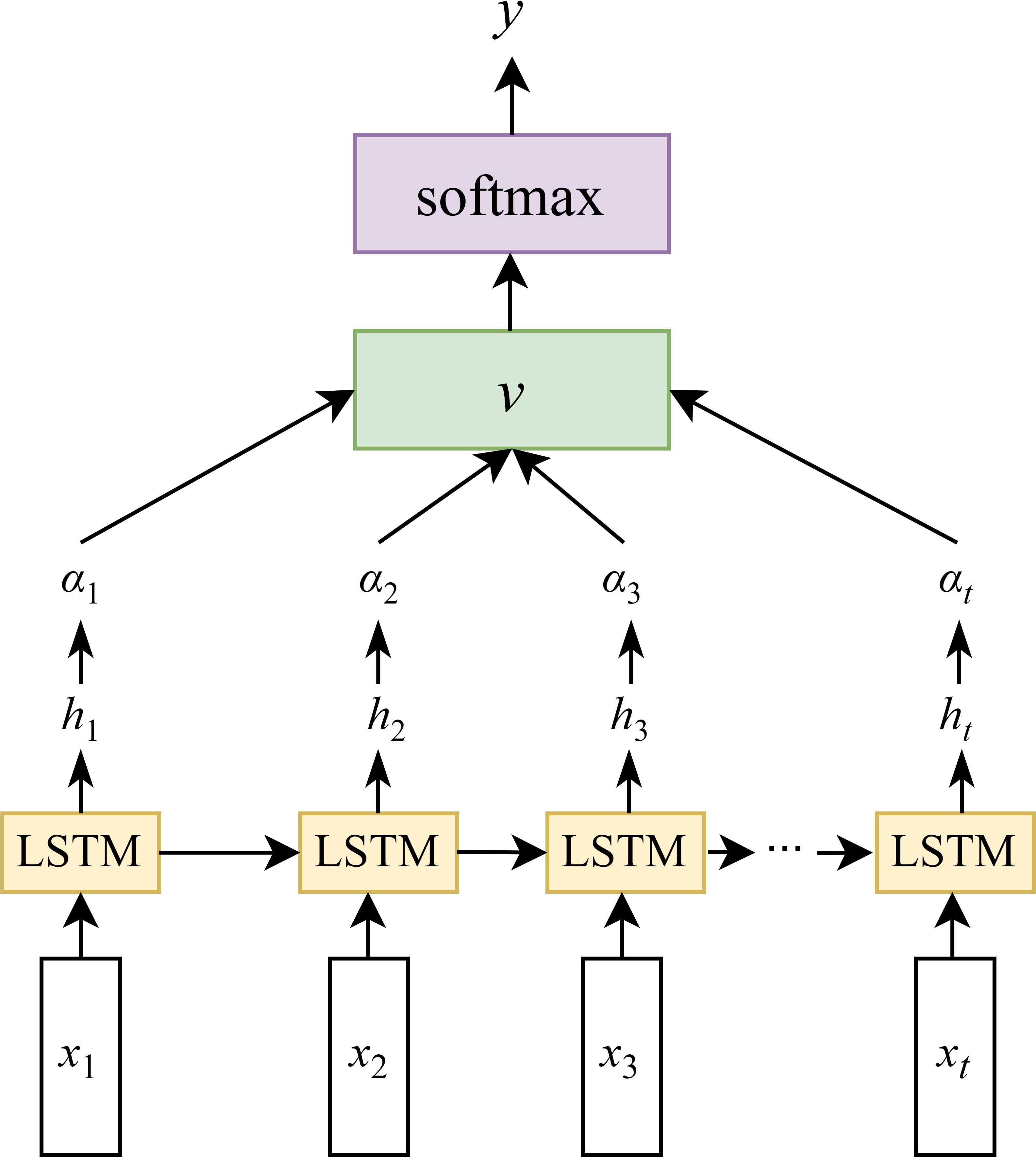
Figure 6. The LSTM with the introduction of attention.

Moreover, we implemented multiple safeguards against overfitting in our CLA model: (1) dropout layers (rate=0.3) after each LSTM and dense layer; (2) L2 weight regularization (λ = 0.01) on all trainable parameters; (3) early stopping with patience being equal to 10 epochs monitoring validation loss. These measures ensured our final model achieved comparable performance on training (R² = 0.93) and validation (R² = 0.92) sets, indicating effective generalization.

2.6 Technical route and performance assessments

The technical workflow about the rice LAI estimation is illustrated in Figure 7. A sample dataset was constructed by integrating the UAV remote sensing data with time-series LAI. A total of 270 samples were collected and split into a training and validation datasets according to 2:1. In addition to applying deep learning methods (DNN, CNN, LSTM, and CLA) for rice LAI estimation, traditional regression and machine learning algorithms—including linear regression, RFR, PLSR, SVR, and XGBoost—were also employed to benchmark model performance. The model accuracy was evaluated using four metrics: the coefficient of determination (R²), root mean square error (RMSE), mean absolute error (MAE), and relative RMSE (RRMSE). The following are the pertinent calculation formulas (Equations 4–7):

Figure 7

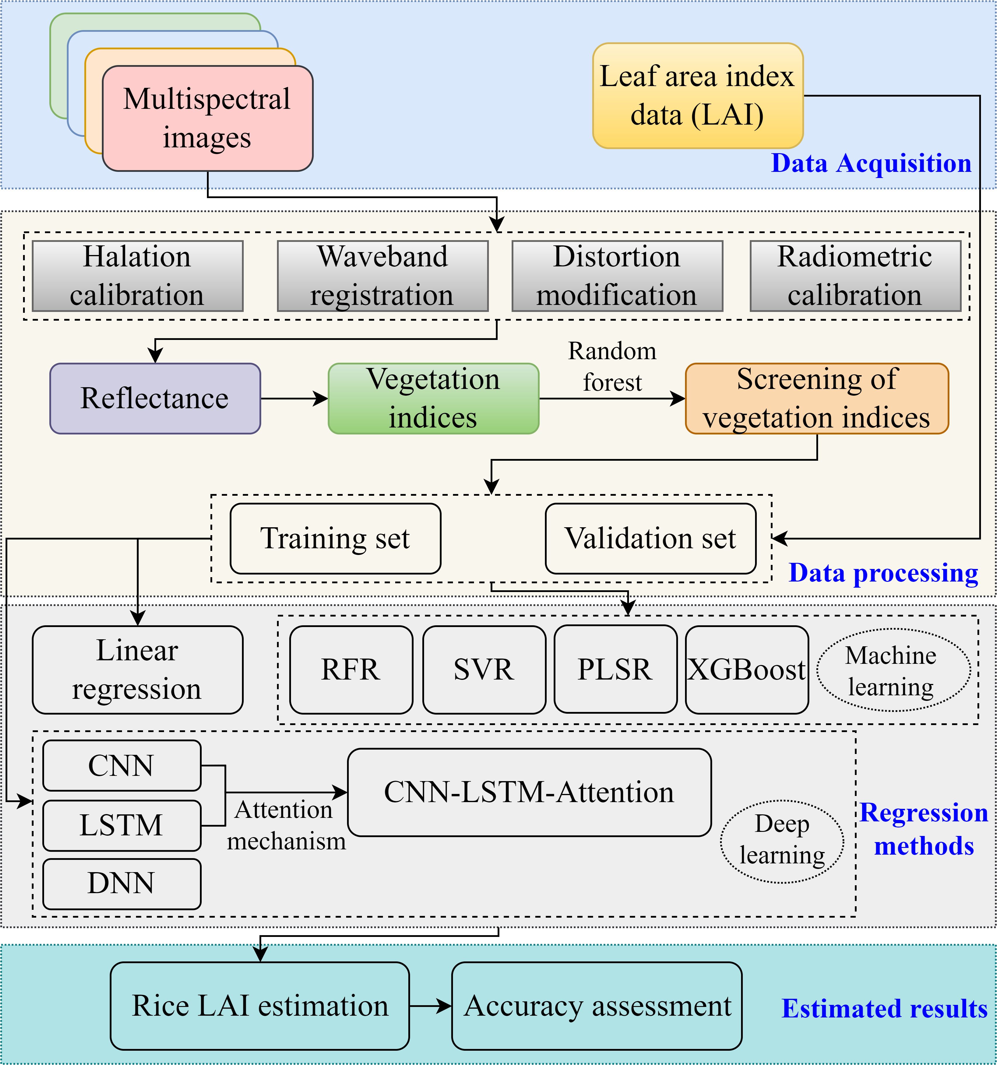
Figure 7. Technical route for LAI estimation in rice.

$\begin{array}{ll}\begin{array}{c}{R}^2= 1- \frac{{\sum }_{i=1}^n{(y-\widehat{y})}^2}{{\sum }_{i=1}^n{(y-\overline{y})}^2}\end{array}& (4)\end{array}$

$\begin{array}{ll}\begin{array}{c}RMSE= \sqrt{\frac{{\sum }_{\mathrm{i=1}}^{\text{n}}{(\widehat{y}\text{ - y)}}^2}{\text{n}}}\end{array}& (5)\end{array}$

$\begin{array}{ll}\begin{array}{c}RRMSE= \frac{RMSE}{\overline{y}}\times 100\%\end{array}& (6)\end{array}$

$\begin{array}{ll}\begin{array}{c}MAE= \frac{1}{n}{\sum }_{\mathrm{i=1}}^{\text{n}}\left|y-\widehat{y}\right|\end{array}& (7)\end{array}$

where y, $\widehat{y}$, and $\overline{y}$ stand for the measured, predicted, and average of the measured values, respectively. n is the number of samples.

3 Results and discussion

3.1 Time-series changes in LAI, canopy reflectance, and VIs

The results of the feature importance scores of the 15 vegetation indices calculated based on the random forest approach are shown in Figure 8. Significant differences in the contribution of each index to the model can be found. Among them, NDRE has the highest importance (more than 0.2), followed by NIRv, EVI2, RVI, OSAVI, and NDVI (more than 0.1), respectively, suggesting that these indices have a greater contribution to the target LAI prediction. The remaining nine vegetation indices have lower importance (all below 0.1) and may have limited enhancement to the model performance. Based on the above analysis, we finally selected the top six vegetation indices that are most important for rice LAI prediction for our analysis.

Figure 8

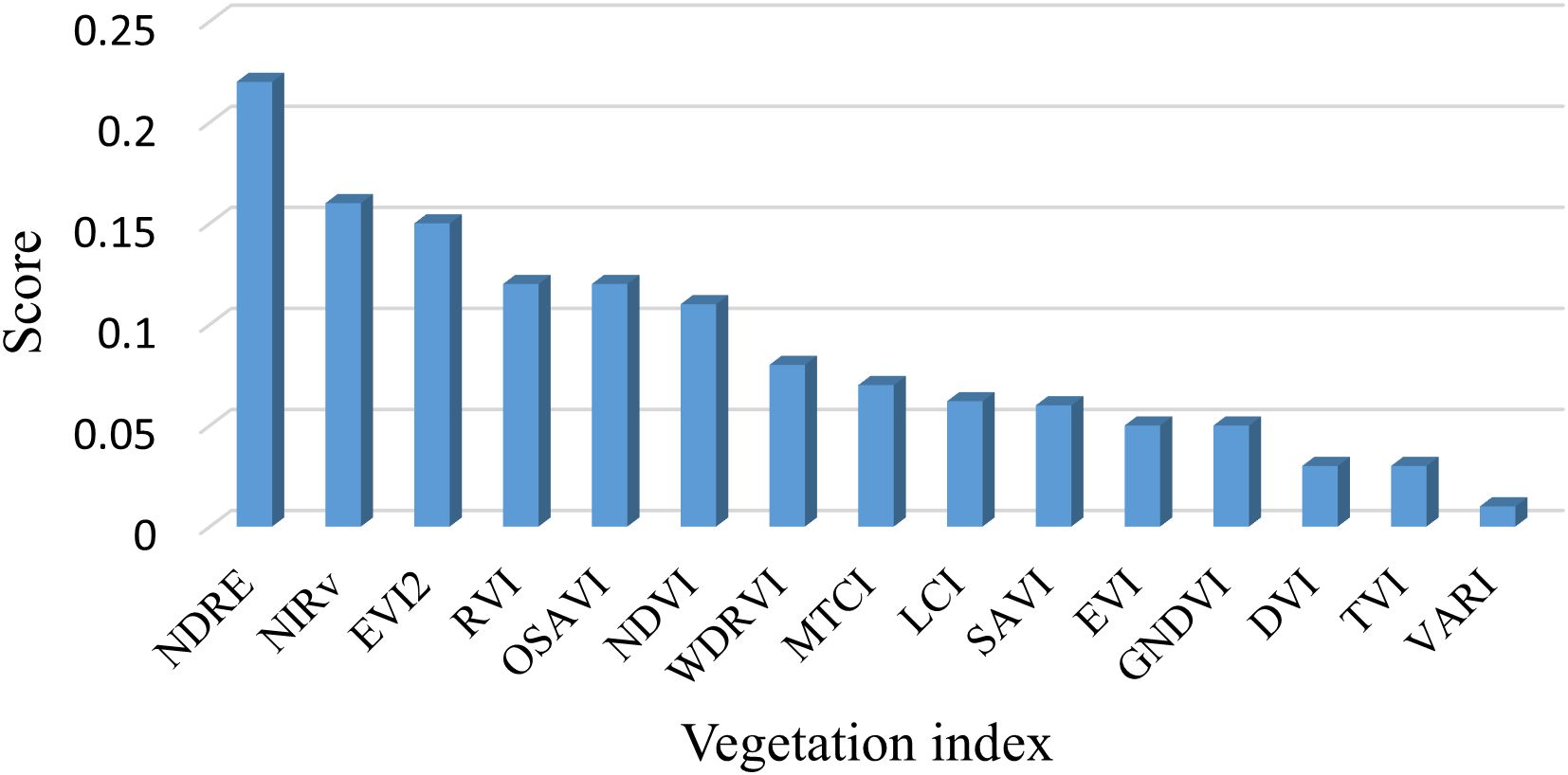
Figure 8. Variable importance ranking based on random forest.

The temporal variation and distribution of rice LAI across ten growth stages are illustrated in Figure 9. Overall, the LAI exhibits a “rise-then-decline” pattern during the rice growing season. This is primarily due to the redistribution of dry matter from vegetative organs (e.g., leaves and stems) to reproductive organs (e.g., panicles) after the booting stage. During the ripening stage, leaf senescence occurs, leading to the gradual yellowing and drying of leaves and consequently a decrease in LAI following its peak (Fang et al., 2014). Taking the case plot shown in Figure 1 as an example, the canopy reflectance at different growth stages is compared in Figure 9. It can be observed that spectral reflectance changes markedly during stages S1 to S3, with only minor fluctuations in subsequent stages. In the near-infrared (NIR) range (842 nm), the reflectance initially increases substantially and then becomes more variable. In the visible band (475-668 nm), the reflectance initially increases substantially and then becomes more variable. In the visible band (490–680 nm), the reflectance generally shows a decreasing trend followed by a slight increase.

Figure 9

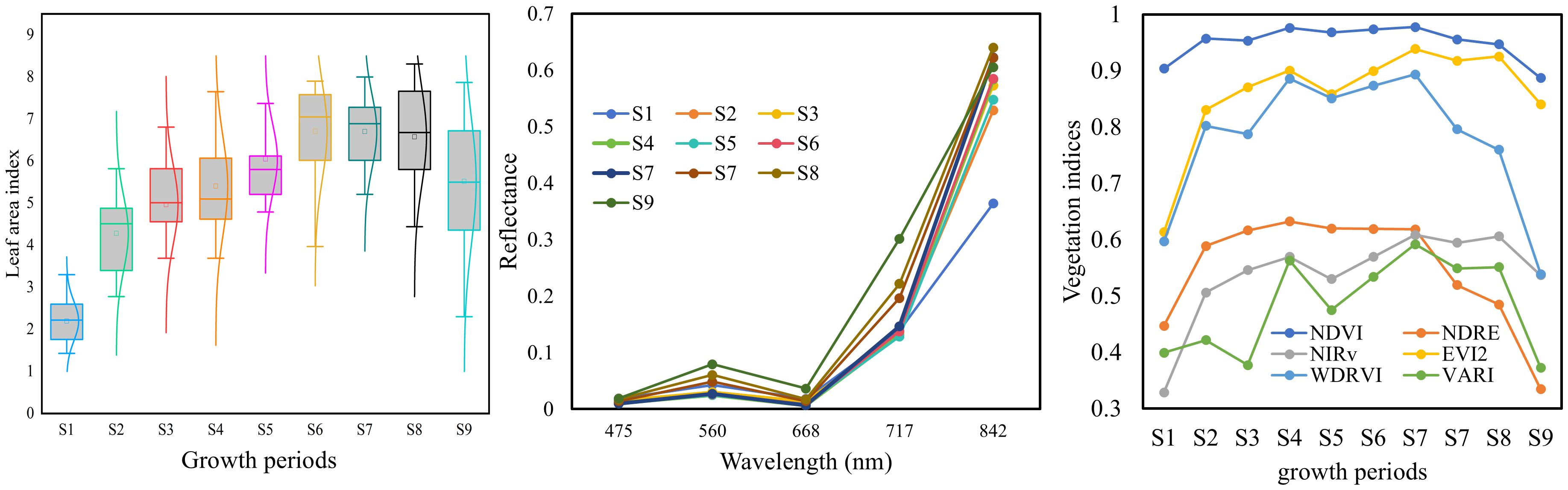
Figure 9. Trends in LAI, canopy reflectance, and vegetation indices in rice.

This variation can be attributed to two main factors: (1) the changing ratio of leaf to soil background throughout the rice growth period; and (2) the intrinsic differences in reflectance between rice plants and bare soil. Specifically, soil has higher reflectance in the visible range but lower reflectance in the NIR band compared to rice vegetation (Luo et al., 2022). Since the rice field consists of a mixture of rice canopy and soil, the composition and proportion of these components vary over time. Shortly after transplanting, the canopy is dominated by exposed soil. As tillering and vegetative growth progress, rice becomes the dominant component. From booting to heading stages, the emergence of panicles further alters the canopy composition. These dynamic changes in field components lead to complex variations in canopy spectra, which can affect the accuracy of optical remote sensing for rice growth parameter estimation (Duan et al., 2019; Wang et al., 2021).

By combining different spectral bands, VIs enhance sensitivity to specific crop parameters while reducing the influence of confounding factors (Verrelst et al., 2015). Numerous indices have been developed to minimize such disturbances, including background soil reflectance, leaf pigment content, leaf water content, leaf inclination angle, atmospheric conditions, and structural parameters of leaves or canopies (Huete, 1988; Rondeaux et al., 1996; Cao et al., 2017; Fang et al., 2017). However, the performance of VIs can vary under different conditions. For example, the NDVI is highly sensitive to soil background when LAI is low (Shang et al., 2015), and it tends to saturate at high LAI values, losing sensitivity as LAI increases (Liu et al., 2012). The temporal variation in VIs during the rice growth period is shown in Figure 9. Compared to reflectance, the temporal trends of VIs exhibit more consistent patterns, with most VIs increasing initially and then decreasing. Among them, NDVI and OSAVI exhibit the most pronounced saturation. Overall, the trajectories of VIs align more closely with those of LAI, suggesting their potential for LAI estimation.

3.2 Estimation of rice LAI based on different VIs

A linear regression model was employed to estimate rice LAI across all growth stages based on individual VIs selected in this study. The results are presented in Figure 10. Except for RVI, the other VIs yielded similar estimation accuracy, with R² values around 0.52 and RRMSE slightly above 20%. Among these, EVI2 produced the highest estimation accuracy, with R² = 0.58, RMSE = 1.18, MAE = 0.99, and RRMSE = 20.24%. However, notable deviations from the 1:1 line were observed in the LAI predictions for NDVI and RVI at low LAI values (0-4), and saturation occurred at high LAI values (> 4), where predicted values varied little despite increases in measured LAI. This is because, in the mid-to-late growth stages, canopy closure reduces red band reflectance changes while NIR reflectance remains high, leading to VI saturation (Gu et al., 2013). In contrast, NIRv performed better for high LAI but showed clear underestimation for low LAI values, likely due to soil background influence on NIR reflectance when the canopy is sparse (Darvishzadeh et al., 2008). NDRE demonstrated similar behavior to NIRv, but its estimates at low LAI were slightly more accurate due to its reduced sensitivity to soil background (Deng et al., 2018). Compared to NDVI, NIRv, OSAVI, NDRE, and RVI, EVI2 performed slightly better across both low and high LAI ranges, indicating its potential in reducing background noise and mitigating saturation (Liu et al., 2012). These results suggest that linear regression with single VIs is insufficient for accurately estimating rice LAI across all growth stages.

Figure 10

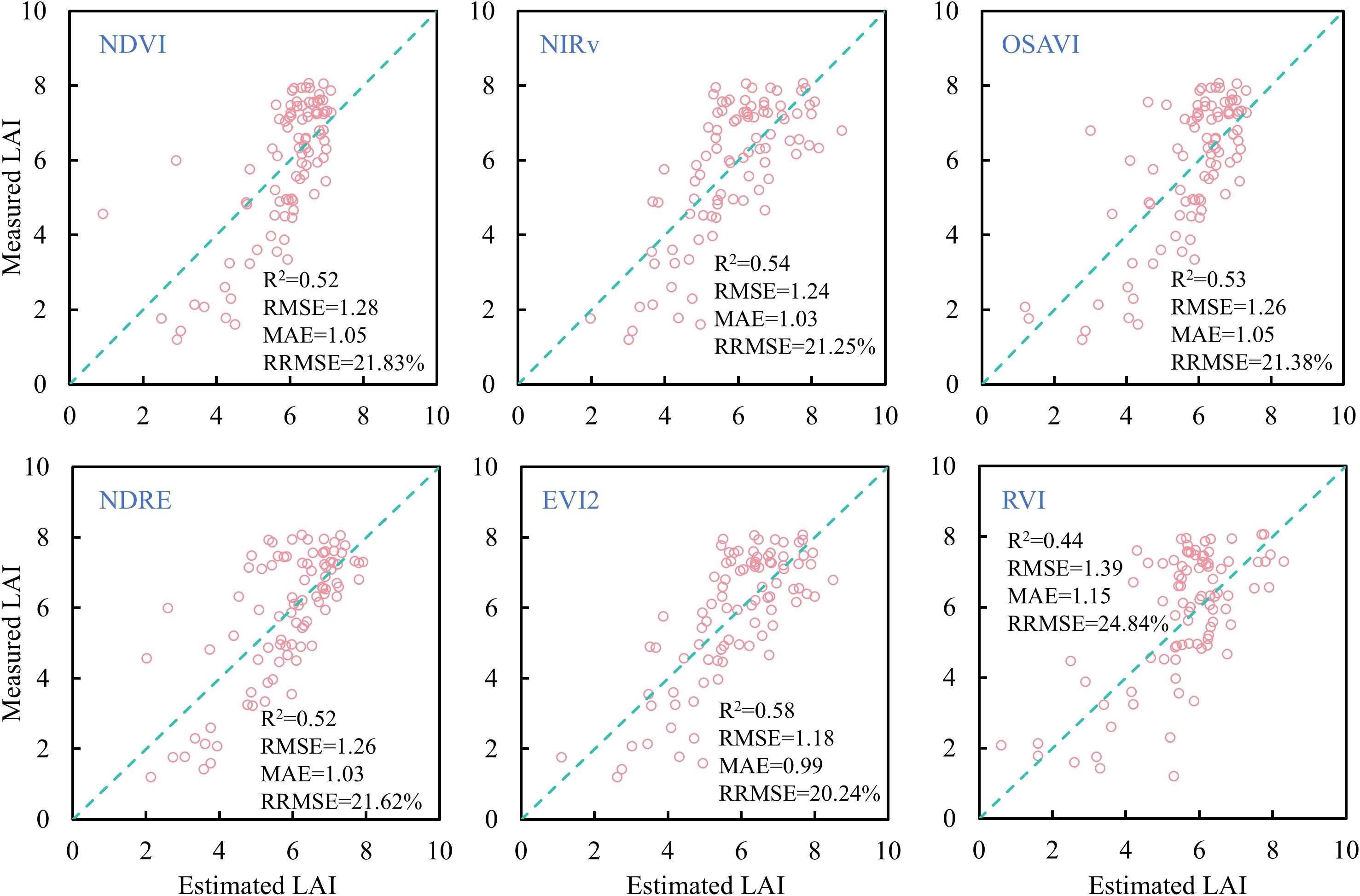
Figure 10. Comparison of rice LAI estimation results based on different vegetation indices.

3.3 Machine learning-based estimation of LAI in rice

In addition to simple linear regression and traditional multivariate regression methods (e.g., multiple linear regression and stepwise regression), machine learning demonstrates distinct advantages in multi-variable integration and nonlinear modeling. For instance, by integrating data from multiple sensors, the RFR method achieved high accuracy in estimating cotton LAI, with R² = 0.95 and RMSE = 0.33 (Yan et al., 2022). When comparing SVR, RFR, and XGBoost for estimating jointing-stage winter wheat LAI using fused spectral, texture, and height data, XGBoost exhibited the highest performance (R² = 0.88, RMSE = 0.69) (Zou et al., 2024). Although various machine learning approaches have achieved relatively high estimation accuracy, most studies rely on multi-source sensors (e.g., RGB, multispectral, hyperspectral, and LiDAR) or heterogeneous variable types (e.g., spectral, texture, and structural features), which not only increase equipment and computational costs, but also reduce interpretability, especially for texture-based metrics.

In this study, SVR, RFR, PLSR, and XGBoost were applied to estimate rice LAI across the entire growing season. The results (Figure 11) indicate that, compared with simple linear regression, machine learning algorithms significantly improved estimation accuracy. Among them, SVR and PLSR showed limited improvements, while RFR and XGBoost yielded more notable performance gains. Of the four tested machine learning algorithms, RFR achieved the highest accuracy for full-season LAI estimation (R² = 0.81, RRMSE< 14%), representing an approximate 6% improvement in RRMSE over linear models using individual VIs.

Figure 11

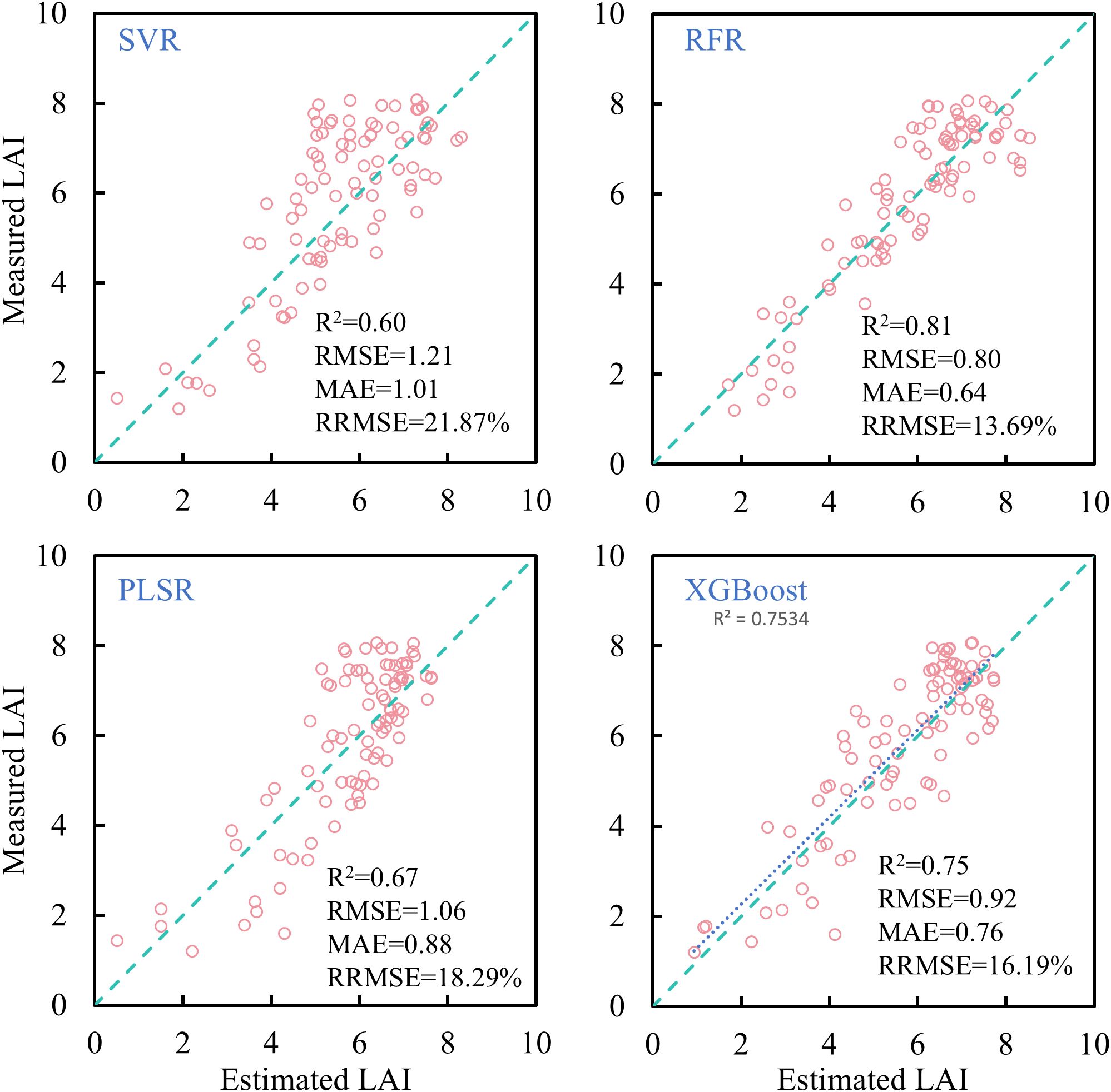
Figure 11. Comparison of rice LAI estimation results based on different machine learning methods.

3.4 Deep learning-based estimation of LAI in rice

Deep learning, a rapidly emerging subfield of machine learning, constructs hierarchical models by simulating biological neural networks, enabling automatic feature extraction and learning from complex datasets (Yue et al., 2024; Liu et al., 2021). Compared to conventional machine learning methods, deep learning models offer superior feature extraction and generalization capabilities, particularly for high-dimensional and heterogeneous data (Liu et al., 2025; Yue et al., 2024). Fully connected neural networks (FCNNs) are a typical deep learning architecture where each neuron is connected to all neurons in the preceding layer, allowing the model to learn intricate patterns and features (Jia and Zhang, 2023). With the development of CNNs, it has become feasible to extract deeper image features, making CNN-based approaches particularly effective for LAI estimation (Yang et al., 2025).

In this study, four deep learning models, DNN, LSTM, CNN, and CLA, were employed to estimate rice LAI across the full growth period. As shown in Figure 12, compared to linear regression and most machine learning models (except RFR), deep learning models substantially improved LAI estimation accuracy. The CLA model achieved the best performance (R² = 0.92, RRMSE< 9%), while other deep learning models exhibited estimation errors above 10%. Notably, not all deep learning models outperformed traditional machine learning: both DNN and LSTM showed lower accuracy than RFR, with estimation errors exceeding 15%, compared to<14% for RFR. CNN yielded higher accuracy than all machine learning models, though lower than CLA. Additionally, deep learning models demonstrated superior performance in estimating both low and high LAI values.

Figure 12

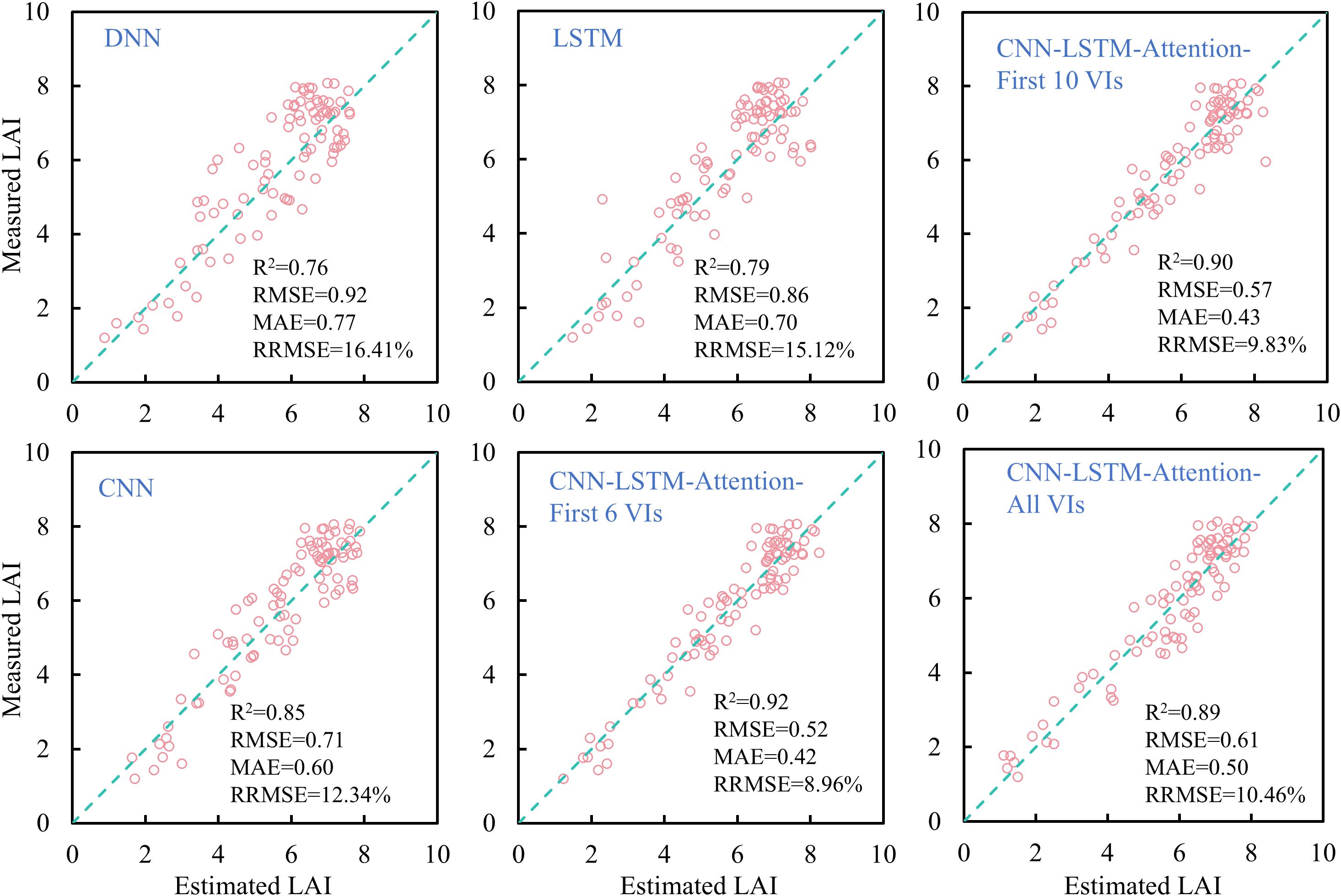
Figure 12. Comparison of rice LAI estimation results based on different deep learning models.

Previous studies have shown that DNN models outperformed PLSR, SVR, and RFR when estimating maize LAI using multi-modal UAV data (RGB, multispectral, and thermal infrared), achieving R² = 0.89 and RRMSE = 12.92% (Liu et al., 2021). The integration of canopy spectral, structural, thermal, and texture features from multi-sensor UAV imagery has also demonstrated the advantages of DNNs in soybean yield estimation (Maimaitijiang et al., 2020). Moreover, combining vegetation indices, texture, and VI-derived deep features through a deep learning model (ResNet50) has further improved maize LAI estimation accuracy (Qiao et al., 2022). These findings suggest that leveraging structural and multi-modal data beyond spectral features holds great potential for enhancing rice LAI estimation accuracy, warranting further investigation.

Furthermore, in order to explore the effect of different VI combinations on the accuracy of deep learning models. We respectively take the top six, top ten and top fifteen VIs in the importance ranking as the inputs to the CLA model, and a comparison of the results is shown in Figure 12. It can be found that it is not the case that the more input variables, the higher the model accuracy. After filtering the importance of variables, the CLA model obtained the highest accuracy of rice LAI prediction when the first six VIs were used as inputs. When the VIs increased, the model accuracy gradually decreased. When all VIs were input, the model accuracy was the lowest. The above results indicate that redundant variables negatively affect the accuracy of deep learning models. Therefore, the screening of input variables is necessary when fusing multivariate features.

3.5 Comparison of model performance with existing studies

The proposed CLA model demonstrated superior performance in rice LAI estimation compared to existing approaches. As shown in Table 3, our model achieved an R² of 0.92 and RRMSE of 8.96%, outperforming previous studies using similar UAV data. For instance, the maize LAI predicted was reported R²=0.89 and RRMSE=12.92% with a DNN model by fusing multimodal remote sensing data (RGB + multispectral + thermal infrared) (Liu et al., 2021), while another maize LAI estimation study obtained R²=0.87 using texture-enhanced vegetation indices (Zhang et al., 2022). Few studies have obtained high LAI estimation accuracy using only multispectral remote sensing data. These comparisons confirm that the CLA framework advances the state-of-the-art in crop LAI estimation, while maintaining computational efficiency suitable for operational agricultural monitoring. However, cross-validation across different geographical regions and growing seasons remains necessary to fully assess its generalization capability. The performance improvement of the CLA model can be attributed to three key factors: (1) the effective integration of spatial-temporal features through CNN-LSTM architecture; (2) the attention mechanism’s ability to weight critical growth stages; and (3) comprehensive coverage of all phenological stages in model training.

Table 3

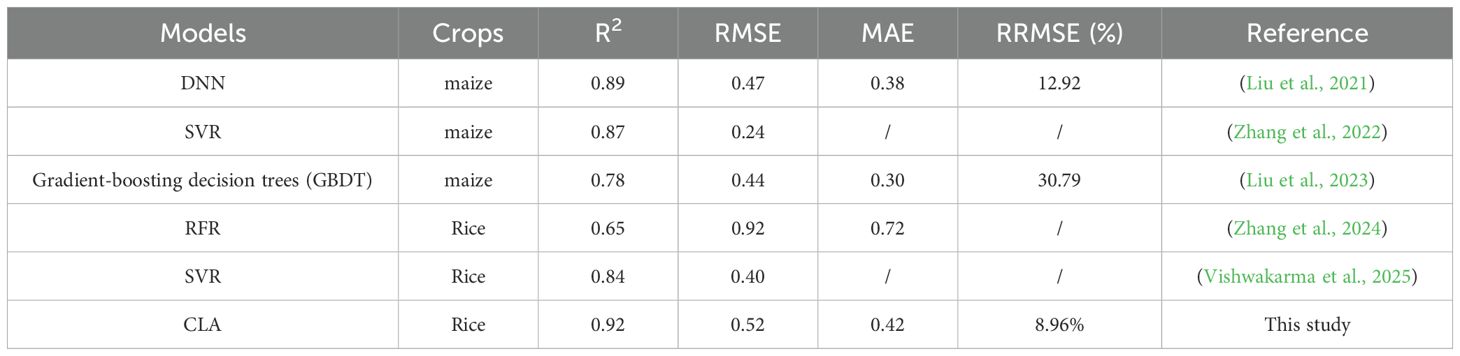
Table 3. Comparison of the performance of the LAI estimation model in this study with the accuracy in existing studies.

3.6 Comparison of estimation accuracy

To further compare the performance of different models in estimating full-season rice LAI, a comprehensive comparison of accuracy metrics is presented in Figure 13. Among the screening vegetation indices, NDVI, NIRv, OSAVI, NDRE, and EVI2 showed similar performance (R² ≈ 0.5, RMSE ≈ 1.3, MAE ≈ 1, RRMSE ≈ 22%), while RVI performed slightly poorly. Among machine learning methods, RFR showed the best performance (R² = 0.81, RMSE< 1, MAE ≈ 0.6, RRMSE< 14%), while other machine learning algorithms performed comparably. Overall, machine learning significantly outperformed linear regression models based on individual vegetation indices. Among deep learning models, CLA achieved the highest accuracy (R² = 0.92, RMSE< 0.6, MAE< 0.5, RRMSE< 9%), while other deep learning models performed similarly to RFR. These results demonstrate the superior capability of deep learning models in capturing nonlinear and spatiotemporal patterns in rice LAI estimation.

Figure 13

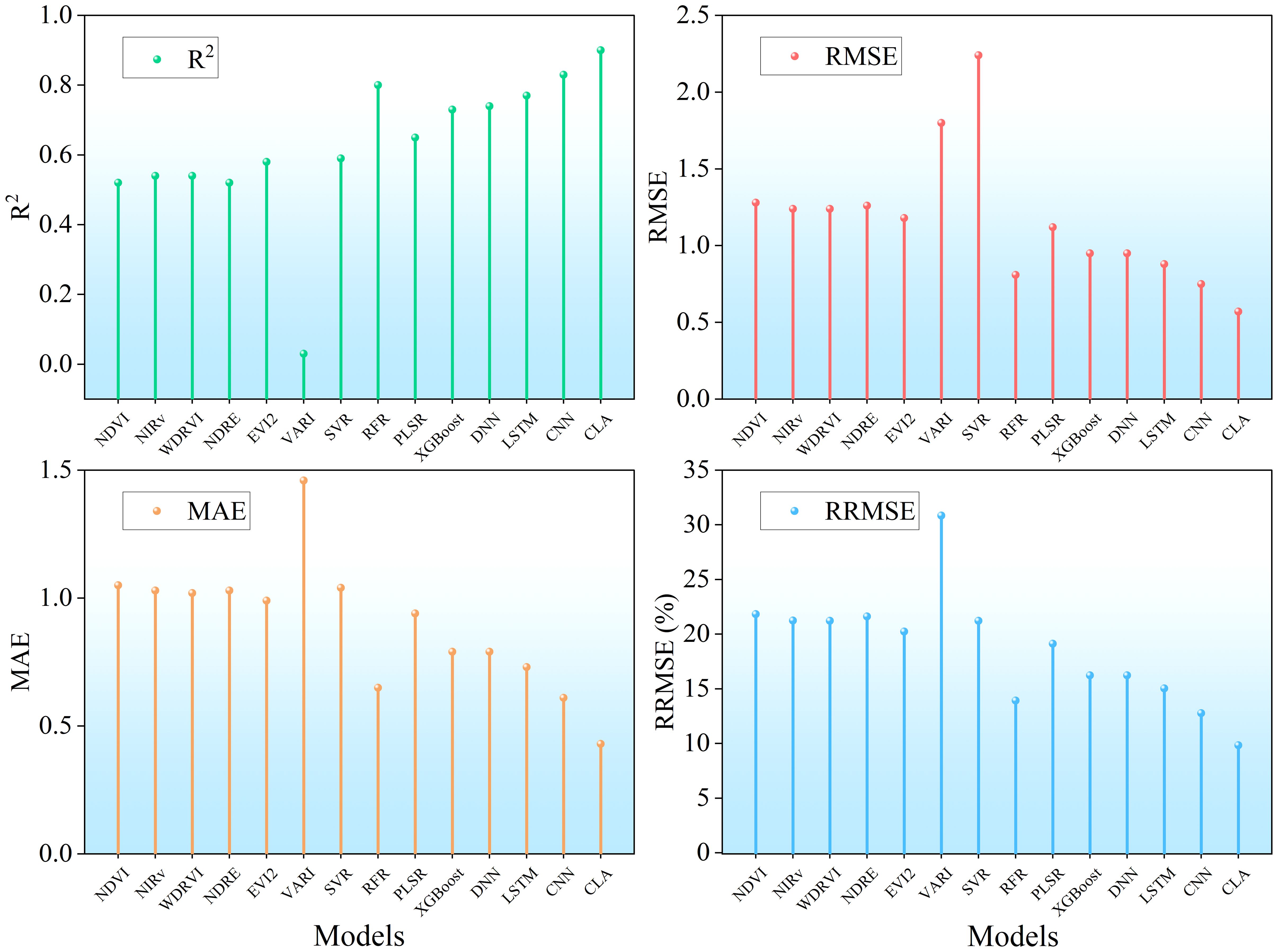
Figure 13. Comparison of LAI estimation accuracy in rice.

To evaluate model performance across different LAI ranges, measured LAI values were stratified into three groups: low (1-3), medium (3-6), and high (6-10). Estimation errors for each range are shown in Figure 14. When LAI< 3, simple linear regression based on most vegetation indices produced errors exceeding 100%. In contrast, all machine learning models achieved errors< 80%, with RFR achieving< 50%. Deep learning models performed even better, with CLA reducing error to about 20%. For LAI values between 3 and 6, estimation errors were generally below 30% for all methods, around 20% for machine learning models, and below 20% for deep learning models, with CLA again achieving the lowest error (< 15%). In the high LAI range (6-10), model performance slightly declined: linear models yielded about 15% error, machine learning about 13%, and CLA< 8%. Overall, LAI estimation accuracy improved as rice developed, highlighting the robust performance of the proposed CLA model across all growth stages.

Figure 14

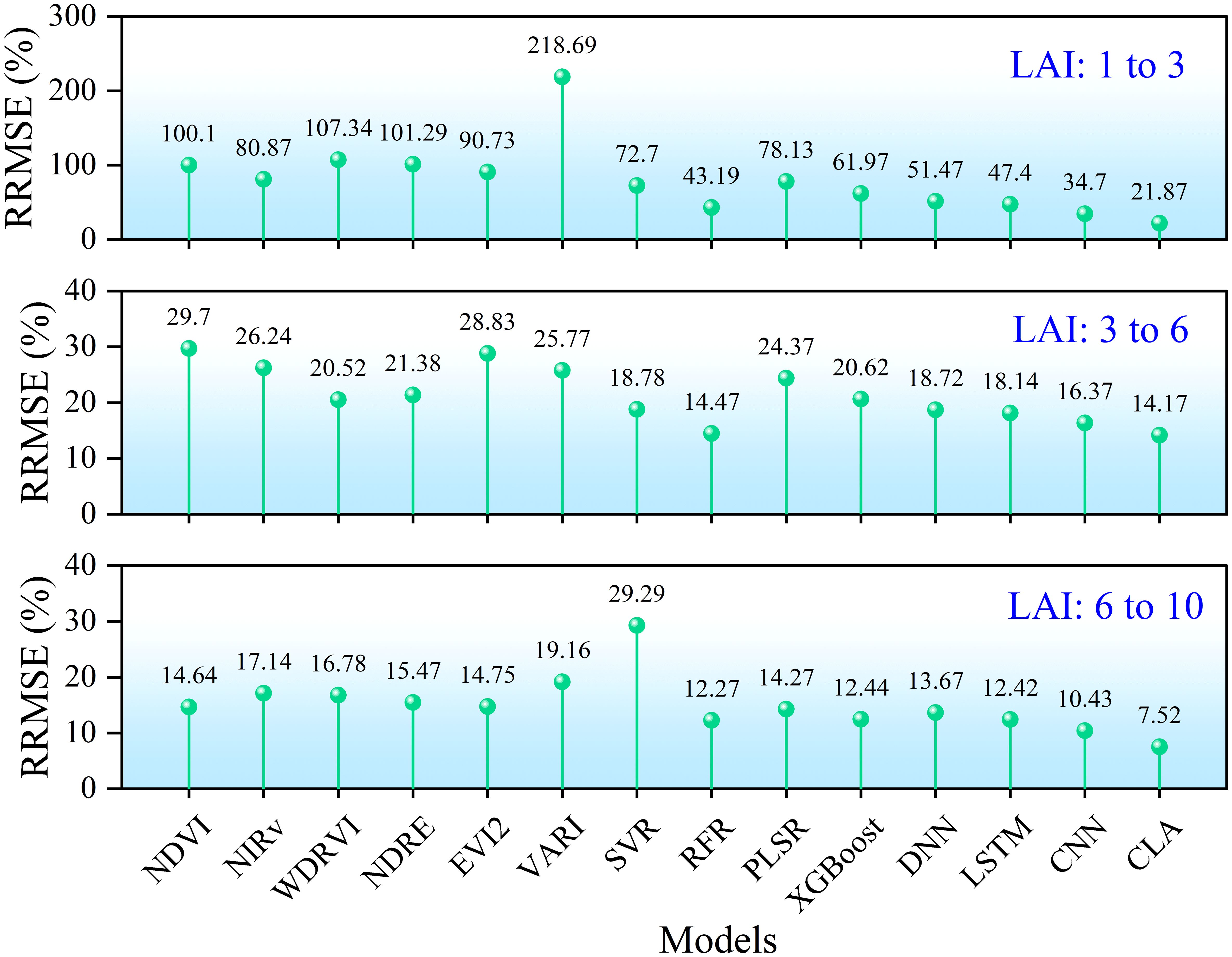
Figure 14. Comparison of estimation errors for refined rice LAI range.

Although this study utilized data covering the entire growing season for model development, a notable limitation is the use of only a single-year dataset, which does not account for interannual variability. Consequently, the model’s generalizability across multiple years remains unverified. To address this limitation, future studies should incorporate multi-season validation, including: (1) testing model performance under different climatic conditions (e.g., drought, excessive rainfall); (2) evaluating robustness against interannual variations in crop management practices; and (3) expanding datasets to include multiple growing seasons to enhance model reliability. This improvement would further strengthen the model’s applicability in precision agriculture under varying environmental conditions.

4 Conclusions

This study developed a CLA model based on UAV multispectral imagery and deep learning techniques to achieve high-accuracy estimation of rice LAI across all growth stages. Comparative analyses were conducted against traditional vegetation index-based regression and machine learning methods. The main conclusions are as follows:

1. The proposed CLA model effectively integrates CNN, LSTM, and an attention mechanism to capture the spatiotemporal features of canopy spectral data. It significantly improves the accuracy of full-season LAI estimation (R² = 0.92, RRMSE< 9%), outperforming traditional linear regression and individual machine learning models.

2. Linear regression models based on vegetation indices are limited by soil background effects and saturation issues, yielding relatively low estimation accuracy (R² ≈ 0.5). Although machine learning methods such as RFR show improved performance (R² = 0.81), deep learning models, particularly CLA, demonstrate superior capability in modeling nonlinear relationships and enhancing generalization.

3. The CLA model exhibits robust performance across different LAI ranges. Notably, it achieves the lowest estimation error (~20%) in the low LAI range (1-3), effectively addressing the challenges faced by traditional approaches during early growth stages and in dense canopy conditions.

Subsequent studies should investigate the merging of multimodal data (e.g., hyperspectral and LiDAR) with deep learning models to further enhance estimation robustness under complex conditions. In addition, optimizing lightweight model architectures will be essential for facilitating practical deployment in agricultural monitoring.

Data availability statement

The original contributions presented in the study are included in the article/supplementary material. Further inquiries can be directed to the corresponding author.

Author contributions

HL: Writing – original draft, Validation, Conceptualization, Project administration, Methodology. LY: Software, Writing – review & editing, Formal analysis, Methodology. SL: Resources, Funding acquisition, Writing – review & editing, Investigation, Data curation, Conceptualization, Validation.

Funding

The author(s) declare financial support was received for the research and/or publication of this article. This research was funded by Joint Fund of Henan Province Science and Technology R&D Program, grant number 235200810069, Science and Technology Tackling Project of Henan Province, grant numbers 242102210011 and 242102210069, Basic Research Operating Expenses Program of Henan Academy of Sciences, grant number 240625002, Scientific Research Initiation Program for High-level Talents of Henan Academy of Sciences, grant number 241825015. The 10th Batch of Key Disciplines in Henan Province: “Electronic Information”.

Conflict of interest

The authors declare that the research was conducted in the absence of any commercial or financial relationships that could be construed as a potential conflict of interest.

Generative AI statement

The authors declare that no Generative AI was used in the creation of this manuscript.

Any alternative text (alt text) provided alongside figures in this article has been generated by Frontiers with the support of artificial intelligence and reasonable efforts have been made to ensure accuracy, including review by the authors wherever possible. If you identify any issues, please contact us.

Publisher’s note

All claims expressed in this article are solely those of the authors and do not necessarily represent those of their affiliated organizations, or those of the publisher, the editors and the reviewers. Any product that may be evaluated in this article, or claim that may be made by its manufacturer, is not guaranteed or endorsed by the publisher.

References

Badgley, G., Field, C. B., and Berry, J. A. (2017). Canopy near-infrared reflectance and terrestrial photosynthesis. Sci. Adv. 3, 5. doi: 10.1126/sciadv.1602244

PubMed Abstract | Crossref Full Text | Google Scholar

Bhadra, S., Sagan, V., Sarkar, S., Braud, M., Mockler, T. C., and Eveland, A. L. (2024). PROSAIL-Net: A transfer learning-based dual stream neural network to estimate leaf chlorophyll and leaf angle of crops from UAV hyperspectral images. Isprs J. Photogrammetry Remote Sens. 210, 1–24. doi: 10.1016/j.isprsjprs.2024.02.020

Crossref Full Text | Google Scholar

Broge, N. H. and Leblanc, E. (2001). Comparing prediction power and stability of broadband and hyperspectral vegetation indices for estimation of green leaf area index and canopy chlorophyll density. Remote Sens. Environ. 76, 156–172. doi: 10.1016/S0034-4257(00)00197-8

Crossref Full Text | Google Scholar

Cao, Z. S., Cheng, T., Ma, X., Tian, Y. C., Zhu, Y., Yao, X., et al. (2017). A new three-band spectral index for mitigating the saturation in the estimation of leaf area index in wheat. Int. J. Remote Sens. 38, 3865–3885. doi: 10.1080/01431161.2017.1306141

Crossref Full Text | Google Scholar

Chen, J. M. and Black, T. A. (1992). Defining leaf-area index for non-flat leaves. Plant Cell Environ. 15, 421–429. doi: 10.1111/j.1365-3040.1992.tb00992.x

Crossref Full Text | Google Scholar

Choi, H., Cho, K., and Bengio, Y. (2018). Fine-grained attention mechanism for neural machine translation. Neurocomputing 284, 171–176. doi: 10.1016/j.neucom.2018.01.007

Crossref Full Text | Google Scholar

Clevers, J. G. P. W. and Gitelson, A. A. (2013). Remote estimation of crop and grass chlorophyll and nitrogen content using red-edge bands on Sentinel-2 and-3. Int. J. Appl. Earth Observation Geoinformation 23, 344–351. doi: 10.1016/j.jag.2012.10.008

Crossref Full Text | Google Scholar

Danson, F. M., Rowland, C. S., and Baret, F. (2003). Training a neural network with a canopy reflectance model to estimate crop leaf area index. Int. J. Remote Sens. 24, 4891–4905. doi: 10.1080/0143116031000070319

Crossref Full Text | Google Scholar

Darvishzadeh, R., Skidmore, A., Atzberger, C., and van Wieren, S. (2008). Estimation of vegetation LAI from hyperspectral reflectance data: Effects of soil type and plant architecture. Int. J. Appl. Earth Observation Geoinformation 10, 358–373. doi: 10.1016/j.jag.2008.02.005

Crossref Full Text | Google Scholar

Dash, J. and Curran, P. J. (2004). The MERIS terrestrial chlorophyll index. Int. J. Remote Sens. 25, 5403–5413. doi: 10.1080/0143116042000274015

Crossref Full Text | Google Scholar

Datt, B. (1999). A new reflectance index for remote sensing of chlorophyll content in higher plants:: Tests using Eucalyptus leaves. J. Plant Physiol. 154, 30–36. doi: 10.1016/S0176-1617(99)80314-9

Crossref Full Text | Google Scholar

Delegido, J., Verrelst, J., Meza, C. M., Rivera, J. P., Alonso, L., and Moreno, J. (2013). A red-edge spectral index for remote sensing estimation of green LAI over agroecosystems. Eur. J. Agron. 46, 42–52. doi: 10.1016/j.eja.2012.12.001

Crossref Full Text | Google Scholar

Deng, L., Mao, Z. H., Li, X. J., Hu, Z. W., Duan, F. Z., and Yan, Y. N. (2018). UAV-based multispectral remote sensing for precision agriculture: A comparison between different cameras. Isprs J. Photogrammetry Remote Sens. 146, 124–136. doi: 10.1016/j.isprsjprs.2018.09.008

Crossref Full Text | Google Scholar

Dhaka, P. and Nagpal, B. (2023). WoM-based deep BiLSTM: smart disease prediction model using WoM-based deep BiLSTM classifier. Multimedia Tools Appl. 82, 25061–25082. doi: 10.1007/s11042-023-14336-x

Crossref Full Text | Google Scholar

Du, J. L., Zhang, Y., Wang, P. X., Tansey, K., Liu, J. M., and Zhang, S. Y. (2025). Enhancing winter wheat yield estimation with a CNN-Transformer hybrid framework utilizing multiple remotely sensed parameters. IEEE Trans. Geosci. Remote Sens. 63, 13. doi: 10.1109/TGRS.2025.3544434

Crossref Full Text | Google Scholar

Duan, B., Liu, Y. T., Gong, Y., Peng, Y., Wu, X. T., Zhu, R. S., et al. (2019). Remote estimation of rice LAI based on Fourier spectrum texture from UAV image. Plant Methods 15, 12. doi: 10.1186/s13007-019-0507-8

PubMed Abstract | Crossref Full Text | Google Scholar

Fang, H. L., Baret, F., Plummer, S., and Schaepman-Strub, G. (2019). An overview of global leaf area index (LAI): Methods, Products, Validation, and Applications. Rev. Geophysics 57, 739–799. doi: 10.1029/2018RG000608

Crossref Full Text | Google Scholar

Fang, H. L., Li, W. J., Wei, S. S., and Jiang, C. Y. (2014). Seasonal variation of leaf area index (LAI) over paddy rice fields in NE China: Intercomparison of destructive sampling, LAI-2200, digital hemispherical photography (DHP), and AccuPAR methods. Agric. For. Meteorology 198, 126–141. doi: 10.1016/j.agrformet.2014.08.005

Crossref Full Text | Google Scholar

Fang, M. H., Ju, W. M., Zhan, W. F., Cheng, T., Qiu, F., and Wang, J. (2017). A new spectral similarity water index for the estimation of leaf water content from hyperspectral data of leaves. Remote Sens. Environ. 196, 13–27. doi: 10.1016/j.rse.2017.04.029

Crossref Full Text | Google Scholar

Gitelson, A. A. (2004). Wide dynamic range vegetation index for remote quantification of biophysical characteristics of vegetation. J. Plant Physiol. 161, 165–173. doi: 10.1078/0176-1617-01176

PubMed Abstract | Crossref Full Text | Google Scholar

Gitelson, A. A., Gritz, Y., and Merzlyak, M. N. (2003). Relationships between leaf chlorophyll content and spectral reflectance and algorithms for non-destructive chlorophyll assessment in higher plant leaves. J. Plant Physiol. 160, 271–282. doi: 10.1078/0176-1617-00887

PubMed Abstract | Crossref Full Text | Google Scholar

Gitelson, A. A., Kaufman, Y. J., and Merzlyak, M. N. (1996). Use of a green channel in remote sensing of global vegetation from EOS-MODIS. Remote Sens. Environ. 58, 289–298. doi: 10.1016/S0034-4257(96)00072-7

Crossref Full Text | Google Scholar

Gitelson, A. A., Kaufman, Y. J., Stark, R., and Rundquist, D. (2002). Novel algorithms for remote estimation of vegetation fraction. Remote Sens. Environ. 80, 76–87. doi: 10.1016/S0034-4257(01)00289-9

Crossref Full Text | Google Scholar

Gitelson, A. and Merzlyak, M. N. (1994). Quantitative estimation of chlorophyll-a using reflectance spectra - experiments with autumn chestnut and maple leaves. J. Photochem. Photobiol. B-Biology 22, 247–252. doi: 10.1016/1011-1344(93)06963-4

Crossref Full Text | Google Scholar

Gu, Y. X., Wylie, B. K., Howard, D. M., Phuyal, K. P., and Ji, L. (2013). NDVI saturation adjustment: A new approach for improving cropland performance estimates in the Greater Platte River Basin, USA. Ecol. Indic. 30, 1–6. doi: 10.1016/j.ecolind.2013.01.041

Crossref Full Text | Google Scholar

Guo, Y., Zhang, L. F., He, Y., Cao, S. P., Li, H. Z., Ran, L., et al. (2024). LSTM time series NDVI prediction method incorporating climate elements: A case study of Yellow River Basin, China. J. Hydrology 629, 13. doi: 10.1016/j.jhydrol.2023.130518

Crossref Full Text | Google Scholar

Han, X., Wei, Z., Chen, H., Zhang, B. Z., Li, Y. N., and Du, T. S. (2021). Inversion of winter wheat growth parameters and yield under different water treatments based on UAV multispectral remote sensing. Front. Plant Sci. 12, 13. doi: 10.3389/fpls.2021.609876

PubMed Abstract | Crossref Full Text | Google Scholar

Huete, A. R. (1988). A soil-adjusted vegetation index (SAVI). Remote Sens. Environ. 25, 295–309. doi: 10.1016/0034-4257(88)90106-X

Crossref Full Text | Google Scholar

Jay, S., Maupas, F., Bendoula, R., and Gorretta, N. (2017). Retrieving LAI, chlorophyll and nitrogen contents in sugar beet crops from multi-angular optical remote sensing: Comparison of vegetation indices and PROSAIL inversion for field phenotyping. Field Crops Res. 210, 33–46. doi: 10.1016/j.fcr.2017.05.005

Crossref Full Text | Google Scholar

Jia, B. J. and Zhang, Y. J. (2023). Spectrum analysis for fully connected neural networks. IEEE Trans. Neural Networks Learn. Syst. 34, 10091–10104. doi: 10.1109/TNNLS.2022.3164875

PubMed Abstract | Crossref Full Text | Google Scholar

Jiang, Z. Y., Huete, A. R., Didan, K., and Miura, T. (2008). Development of a two-band enhanced vegetation index without a blue band. Remote Sens. Environ. 112, 3833–3845. doi: 10.1016/j.rse.2008.06.006

Crossref Full Text | Google Scholar

Jordan, C. F. (1969). Derivation of leaf-area index from quality of light on the forest floor. Ecology 50, 663–666. doi: 10.2307/1936256

Crossref Full Text | Google Scholar

Kimes, D. S., Markham, B. L., Tucker, C. J., and McMurtrey, J. E. (1981). Temporal relationships between spectral response and agronomic variables of a corn canopy. Remote Sens. Environ. 11, 401–411. doi: 10.1016/0034-4257(81)90037-7

Crossref Full Text | Google Scholar

Kross, A., McNairn, H., Lapen, D., Sunohara, M., and Champagne, C. (2015). Assessment of RapidEye vegetation indices for estimation of leaf area index and biomass in corn and soybean crops. Int. J. Appl. Earth Observation Geoinformation 34, 235–248. doi: 10.1016/j.jag.2014.08.002

Crossref Full Text | Google Scholar

Li, H. X., Li, Q., Yu, C. L., and Luo, S. J. (2025). Unified estimation of rice canopy leaf area index over multiple periods based on UAV multispectral imagery and deep learning. Plant Methods 21, 16. doi: 10.1186/s13007-025-01398-1

PubMed Abstract | Crossref Full Text | Google Scholar

Li, Y. Y. and Liang, S. L. (2023). Evaluation of reflectance and canopy scattering coefficient based vegetation indices to reduce the impacts of canopy structure and soil in estimating leaf and canopy chlorophyll contents. IEEE Trans. Geosci. Remote Sens. 61, 15. doi: 10.1109/TGRS.2023.3266500

Crossref Full Text | Google Scholar

Li, W. T., Migliavacca, M., Forkel, M., Denissen, J. M. C., Reichstein, M., Yang, H., et al. (2022). Widespread increasing vegetation sensitivity to soil moisture. Nat. Commun. 13, 9. doi: 10.1038/s41467-022-31667-9

PubMed Abstract | Crossref Full Text | Google Scholar

Li, S. Y., Yuan, F., Ata-Ui-Karim, S. T., Zheng, H. B., Cheng, T., Liu, X. J., et al. (2019). Combining color indices and textures of UAV-based digital imagery for rice LAI estimation. Remote Sens. 11, 21. doi: 10.3390/rs11151763

Crossref Full Text | Google Scholar

Liang, L., Di, L. P., Zhang, L. P., Deng, M. X., Qin, Z. H., Zhao, S. H., et al. (2015). Estimation of crop LAI using hyperspectral vegetation indices and a hybrid inversion method. Remote Sens. Environ. 165, 123–134. doi: 10.1016/j.rse.2015.04.032

Crossref Full Text | Google Scholar

Liang, L., Geng, D., Yan, J., Qiu, S. Y., Di, L. P., Wang, S. G., et al. (2020a). Estimating crop LAI using spectral feature extraction and the hybrid inversion method. Remote Sens. 12, 27. doi: 10.3390/rs12213534

Crossref Full Text | Google Scholar

Liang, L., Huang, T., Di, L. P., Geng, D., Yan, J., Wang, S. G., et al. (2020b). Influence of different bandwidths on LAI estimation using vegetation indices. IEEE J. Selected Topics Appl. Earth Observations Remote Sens. 13, 1494–1502. doi: 10.1109/JSTARS.4609443

Crossref Full Text | Google Scholar

Liu, Z. Y., An, R. Z., Qiao, Y. T., Ma, X., Gao, L., and Jin, H. A. (2025). Estimation of leaf area index using radiative transfer process-guided deep learning. IEEE Geosci. Remote Sens. Lett. 22, 5. doi: 10.1109/LGRS.2025.3528181

Crossref Full Text | Google Scholar

Liu, S. B., Jin, X. L., Bai, Y., Wu, W. B., Cui, N. B., Cheng, M. H., et al. (2023). UAV multispectral images for accurate estimation of the maize LAI considering the effect of soil background. Int. J. Appl. Earth Observation Geoinformation 121, 21. doi: 10.1016/j.jag.2023.103383

Crossref Full Text | Google Scholar

Liu, S. B., Jin, X. L., Nie, C. W., Wang, S. Y., Yu, X., Cheng, M. H., et al. (2021). Estimating leaf area index using unmanned aerial vehicle data: shallow vs. deep machine learning algorithms. Plant Physiol. 187, 1551–1576. doi: 10.1093/plphys/kiab322

PubMed Abstract | Crossref Full Text | Google Scholar

Liu, J. G., Pattey, E., and Jégo, G. (2012). Assessment of vegetation indices for regional crop green LAI estimation from Landsat images over multiple growing seasons. Remote Sens. Environ. 123, 347–358. doi: 10.1016/j.rse.2012.04.002

Crossref Full Text | Google Scholar

Luo, S. J., Jiang, X. Q., Yang, K. L., Li, Y. J., and Fang, S. H. (2022). Multispectral remote sensing for accurate acquisition of rice phenotypes: Impacts of radiometric calibration and unmanned aerial vehicle flying altitudes. Front. Plant Sci. 13, 19. doi: 10.3389/fpls.2022.958106

PubMed Abstract | Crossref Full Text | Google Scholar

Ma, Y. R., Zhang, Q., Yi, X., Ma, L. L., Zhang, L. F., Huang, C. P., et al. (2022). Estimation of cotton leaf area index (LAI) based on spectral transformation and vegetation index. Remote Sens. 14, 22. doi: 10.3390/rs14010136

Crossref Full Text | Google Scholar

Maimaitijiang, M., Sagan, V., Sidike, P., Hartling, S., Esposito, F., and Fritschi, F. B. (2020). Soybean yield prediction from UAV using multimodal data fusion and deep learning. Remote Sens. Environ. 237, 20. doi: 10.1016/j.rse.2019.111599

Crossref Full Text | Google Scholar

Murugesan, R., Mishra, E., and Krishnan, A. H. (2022). Forecasting agricultural commodities prices using deep learning-based models: basic LSTM, bi-LSTM, stacked LSTM, CNN LSTM, and convolutional LSTM. Int. J. Sustain. Agric. Manage. Inf. 8, 242–277. doi: 10.1504/IJSAMI.2022.125757

Crossref Full Text | Google Scholar

Qiao, L., Zhao, R. M., Tang, W. J., An, L. L., Sun, H., Li, M. Z., et al. (2022). Estimating maize LAI by exploring deep features of vegetation index map from UAV multispectral images. Field Crops Res. 289, 14. doi: 10.1016/j.fcr.2022.108739

Crossref Full Text | Google Scholar

Rondeaux, G., Steven, M., and Baret, F. (1996). Optimization of soil-adjusted vegetation indices. Remote Sens. Environ. 55, 95–107. doi: 10.1016/0034-4257(95)00186-7

Crossref Full Text | Google Scholar

Roosjen, P. P. J., Brede, B., Suomalainen, J. M., Bartholomeus, H. M., Kooistra, L., and Clevers, J. G. P. W. (2018). Improved estimation of leaf area index and leaf chlorophyll content of a potato crop using multi-angle spectral data - potential of unmanned aerial vehicle imagery. Int. J. Appl. Earth Observation Geoinformation 66, 14–26. doi: 10.1016/j.jag.2017.10.012

Crossref Full Text | Google Scholar

Rouse, J. W., Haas, R. H., Schell, J. A., and Deering, D. W. (1974). Monitoring vegetation systems in the Great Plains with ERTS. NASA Special Publ. 351, 1–9.

Google Scholar

Schlemmer, M., Gitelson, A., Schepers, J., Ferguson, R., Peng, Y., Shanahan, J., et al. (2013). Remote estimation of nitrogen and chlorophyll contents in maize at leaf and canopy levels. Int. J. Appl. Earth Observation Geoinformation 25, 47–54. doi: 10.1016/j.jag.2013.04.003

Crossref Full Text | Google Scholar

Shang, J. L., Liu, J. G., Ma, B. L., Zhao, T., Jiao, X. F., Geng, X. Y., et al. (2015). Mapping spatial variability of crop growth conditions using RapidEye data in Northern Ontario, Canada. Remote Sens. Environ. 168, 113–125. doi: 10.1016/j.rse.2015.06.024

Crossref Full Text | Google Scholar

Sinha, S. K., Padalia, H., Dasgupta, A., Verrelst, J., and Rivera, J. P. (2020). Estimation of leaf area index using PROSAIL based LUT inversion, MLRA-GPR and empirical models: Case study of tropical deciduous forest plantation, North India. Int. J. Appl. Earth Observation Geoinformation 86, 11. doi: 10.1016/j.jag.2019.102027

PubMed Abstract | Crossref Full Text | Google Scholar

Verrelst, J., Camps-Valls, G., Munoz-Mari, J., Rivera, J. P., Veroustraete, F., Clevers, J. G. P. W., et al. (2015). Optical remote sensing and the retrieval of terrestrial vegetation bio-geophysical properties - A review. Isprs J. Photogrammetry Remote Sens. 108, 273–290. doi: 10.1016/j.isprsjprs.2015.05.005

Crossref Full Text | Google Scholar

Vishwakarma, S. K., Bhattarai, B., Kothari, K., and Pandey, A. (2025). Intercomparison of machine learning models for estimating leaf area index of rice using UAV-based multispectral imagery. Phys. Chem. Earth 140, 17. doi: 10.1016/j.pce.2025.103977

Crossref Full Text | Google Scholar

Wang, S. Y., Liu, Y. J., Asseng, S., Harrison, M. T., Tang, L., Liu, B., et al. (2025). Rice yield stability and its determinants across different rice-cropping systems in China. Agric. For. Meteorology 364, 14. doi: 10.1016/j.agrformet.2025.110452

Crossref Full Text | Google Scholar

Wang, W. H., Wu, Y. P., Zhang, Q. F., Zheng, H. B., Yao, X., Zhu, Y., et al. (2021). AAVI: A novel approach to estimating leaf nitrogen concentration in rice from unmanned aerial vehicle multispectral imagery at early and middle growth stages. IEEE J. Selected Topics Appl. Earth Observations Remote Sens. 14, 6716–6728. doi: 10.1109/JSTARS.2021.3086580

Crossref Full Text | Google Scholar

Wang, W. H., Zheng, H. B., Wu, Y. P., Yao, X., Zhu, Y., Cao, W. X., et al. (2022). An assessment of background removal approaches for improved estimation of rice leaf nitrogen concentration with unmanned aerial vehicle multispectral imagery at various observation times. Field Crops Res. 283, 14. doi: 10.1016/j.fcr.2022.108543

Crossref Full Text | Google Scholar

Xu, X. Q., Lu, J. S., Zhang, N., Yang, T. C., He, J. Y., Yao, X., et al. (2019). Inversion of rice canopy chlorophyll content and leaf area index based on coupling of radiative transfer and Bayesian network models. Isprs J. Photogrammetry Remote Sens. 150, 185–196. doi: 10.1016/j.isprsjprs.2019.02.013

Crossref Full Text | Google Scholar

Yan, P. C., Han, Q. S., Feng, Y. M., and Kang, S. Z. (2022). Estimating LAI for cotton using multisource UAV data and a modified universal model. Remote Sens. 14, 22. doi: 10.3390/rs14174272

Crossref Full Text | Google Scholar

Yan, G. J., Hu, R. H., Luo, J. H., Weiss, M., Jiang, H. L., Mu, X. H., et al. (2019). Review of indirect optical measurements of leaf area index: Recent advances, challenges, and perspectives. Agric. For. Meteorology 265, 390–411. doi: 10.1016/j.agrformet.2018.11.033

Crossref Full Text | Google Scholar

Yang, C. K., Lei, J. K., Liu, Z. H., Xiong, S. F., Xi, L., Wang, J., et al. (2025). Estimation model of corn leaf area index based on improved CNN. Agriculture-Basel 15, 20. doi: 10.3390/agriculture15050481

Crossref Full Text | Google Scholar

Yang, G. J., Liu, J. G., Zhao, C. J., Li, Z. H., Huang, Y. B., Yu, H. Y., et al. (2017). Unmanned aerial vehicle remote sensing for field-based crop phenotyping: Current status and perspectives. Front. Plant Sci. 8, 26. doi: 10.3389/fpls.2017.01111

PubMed Abstract | Crossref Full Text | Google Scholar

Yu, F., Bai, J., Fang, J., Guo, S., Zhu, S., and Xu, T. (2024). Integration of a parameter combination discriminator improves the accuracy of chlorophyll inversion from spectral imaging of rice. Agric. Commun. 2, 100055. doi: 10.1016/j.agrcom.2024.100055

Crossref Full Text | Google Scholar

Yuan, H. H., Yang, G. J., Li, C. C., Wang, Y. J., Liu, J. G., Yu, H. Y., et al. (2017). Retrieving soybean leaf area index from unmanned aerial vehicle hyperspectral remote sensing: Analysis of RF, ANN, and SVM regression models. Remote Sens. 9, 14. doi: 10.3390/rs9040309

Crossref Full Text | Google Scholar

Yue, J. B., Feng, H. K., Jin, X. L., Yuan, H. H., Li, Z. H., Zhou, C. Q., et al. (2018). A comparison of crop parameters estimation using images from UAV-mounted snapshot hyperspectral sensor and high-definition digital camera. Remote Sens. 10, 24. doi: 10.3390/rs10071138

Crossref Full Text | Google Scholar

Yue, J., Li, T., Feng, H., Fu, Y., Liu, Y., Tian, J., et al. (2024). Enhancing field soil moisture content monitoring using laboratory-based soil spectral measurements and radiative transfer models. Agric. Commun. 2, 100060. doi: 10.1016/j.agrcom.2024.100060

Crossref Full Text | Google Scholar

Yue, J. B., Tian, J., Philpot, W., Tian, Q. J., Feng, H. K., and Fu, Y. Y. (2023a). VNAI-NDVI-space and polar coordinate method for assessing crop leaf chlorophyll content and fractional cover. Comput. Electron. Agric. 207, 18. doi: 10.1016/j.compag.2023.107758

Crossref Full Text | Google Scholar

Yue, J. B., Wang, J., Zhang, Z. Y., Li, C. C., Yang, H., Feng, H. K., et al. (2024). Estimating crop leaf area index and chlorophyll content using a deep learning-based hyperspectral analysis method. Comput. Electron. Agric. 227, 15. doi: 10.1016/j.compag.2024.109653

Crossref Full Text | Google Scholar

Yue, J. B., Yang, H., Yang, G. J., Fu, Y. Y., Wang, H., and Zhou, C. Q. (2023b). Estimating vertically growing crop above-ground biomass based on UAV remote sensing. Comput. Electron. Agric. 205, 14. doi: 10.1016/j.compag.2023.107627

Crossref Full Text | Google Scholar

Zhang, J. J., Cheng, T., Guo, W., Xu, X., Qiao, H. B., Xie, Y. M., et al. (2021). Leaf area index estimation model for UAV image hyperspectral data based on wavelength variable selection and machine learning methods. Plant Methods 17, 14. doi: 10.1186/s13007-021-00750-5

PubMed Abstract | Crossref Full Text | Google Scholar

Zhang, Y., Jiang, Y. Y., Xu, B., Yang, G. J., Feng, H. K., Yang, X. D., et al. (2024). Study on the estimation of leaf area index in rice based on UAV RGB and multispectral data. Remote Sens. 16, 24. doi: 10.3390/rs16163049

Crossref Full Text | Google Scholar

Zhang, L. C., Sun, B. S., Zhao, D. N., Shan, C. F., Wang, B. J., Wang, G. B., et al. (2024). Improved estimation of cotton (Gossypium hirsutum L.) LAI from multispectral data using UAV point cloud data. Ind. Crops Products 217, 17. doi: 10.1016/j.indcrop.2024.118851

Crossref Full Text | Google Scholar

Zhang, Y., Yang, Y. Z., Zhang, Q. W., Duan, R. Q., Liu, J. Q., Qin, Y. C., et al. (2023). Toward multi-stage phenotyping of soybean with multimodal UAV sensor data: A comparison of machine learning approaches for leaf area index estimation. Remote Sens. 15, 25. doi: 10.3390/rs15010007

Crossref Full Text | Google Scholar

Zhang, X. W., Zhang, K. F., Sun, Y. Q., Zhao, Y. D., Zhuang, H. F., Ban, W., et al. (2022). Combining spectral and texture features of UAS-based multispectral images for maize leaf area index estimation. Remote Sens. 14, 17. doi: 10.3390/rs14020331

Crossref Full Text | Google Scholar

Zhuang, Z. H., Tsai, H. P., Chen, C., and Yang, M. D. (2024). Subtropical region tea tree LAI estimation integrating vegetation indices and texture features derived from UAV multispectral images. Smart Agric. Technol. 9, 17. doi: 10.1016/j.atech.2024.100650

Crossref Full Text | Google Scholar

Zou, M. X., Liu, Y., Fu, M. D., Li, C. J., Zhou, Z. X., Meng, H. R., et al. (2024). Combining spectral and texture feature of UAV image with plant height to improve LAI estimation of winter wheat at jointing stage. Front. Plant Sci. 14, 19. doi: 10.3389/fpls.2023.1272049

PubMed Abstract | Crossref Full Text | Google Scholar