Integrating machine learning and the GGE biplot for identification of climate-suitable grasspea genotypes

Grasspea is a nutrient-rich food legume crop known for its resilience in the challenging agro-ecosystems. However, information is scanty regarding the recommendation of grasspea genotypes with respect to their suitability for both general and specific adaptations. The primary goal of the study was to delineate stable grasspea genotypes by nullifying the influence of intricate interactions among multiple traits with the environment. Additionally, the study aimed to identify suitable locations within diverse agro-climatic zones in India for future evaluation while also validating and predicting results using machine learning algorithms. From several hundred genotypes developed and tested in station trials at Amlaha, India, a panel of 64 diverse promising grasspea genotypes was identified, and their performance was subsequently assessed through multilocation testing at four diverse locations in India during 2021–2022 using the GGE biplot approach. Mean selection index of each genotype was enumerated considering multi-trait performance for better elucidation of genotype and environment ranking as well as selection of the mega-environment. The findings revealed that the environment was the primary contributor to variation across all studied traits, followed by genotype × environment interactions as the second most influential factor. Genotypes such as FLRP-B54-1-S2, Prateek, 31-GP-F3-S7, 31-GP-F3-S4, FLRP-B38-S5, 48-GP-F3-S3, and BANG-288-S2 were identified as good performers with promising multi-trait performance. Experimental results were validated using multiple performance metrics, with the Random Forest (RF) model of machine learning demonstrating superior predictive accuracy compared to the multilayer perceptron (MLP) model. Regression coefficient (R²) values ranged between 0.558 and 0.947, depending on the output variables. In conclusion, “Prateek,” “31-GP-F3-S7,” and “48-GP-F3-S3” emerged as the most stable genotypes when considering their combined yield-trait performance. These genotypes can be recommended for widespread commercial cultivation in regions where grasspea cultivation faces challenges of weather extremities.

Introduction

Grasspea (Lathyrus sativus L.) is a highly adaptable and nutrient-dense cool season food legume crop, cultivated globally in resource-poor dry areas (Mahapatra et al., 2020). Its resilience to varying climates makes it a valuable component for sustainable agriculture and food security in the face of changing climatic conditions (Banerjee et al., 2022; Barpete et al., 2024). This food legume holds significant importance due to its diverse applications in human food, animal feed, and ecosystem management as an input rational crop with an ability to maintain soil health through biological nitrogen fixation. Grasspea is renowned for its high seed protein content (17.7%–49.3%), which boasts an excellent amino acid balance (19.69–23.48 g in 100 g of seed) (Rizvi et al., 2016; Sharma et al., 2022). Notably, the presence of valuable nutraceuticals, such as L-homoarginine, further enhances its nutritional value (Lambein, 2000; Das et al., 2021).

Grasspea is cultivated in rainfed dry regions of Southeast Asia, including India, as well as the Mediterranean, Middle East, and parts of Southern Europe, which are prone to weather whiplashes like the concomitant occurrence of drought and waterlogging (Barpete et al., 2023). The current total area under grasspea cultivation is approximately 0.70 million ha, with a production potential of 0.79 million tons along an average productivity of 1,130 kg per ha (Kumar et al., 2021), The plausible reason behind the decline in area under grasspea cultivation includes the stigma of neurotoxin β-N-oxalyl-L-α,β-diaminopropionic acid (β-ODAP), indeterminate growth habit, and the challenge of maintaining varietal purity due to frequent cross-pollination (Parihar et al., 2022; Tripathi et al., 2022). Identification of early maturing and stable grasspea genotypes that can harmonize optimum vegetative and reproductive growth while maximizing biomass and yield is the most seminal crop breeding property. Lack of comprehensive studies on assessing grasspea genotypes across different locations has created a pressing need to gain a deeper understanding of cultivar behavior under diverse agro-climatic conditions.

Comparing diverse genotypes in multiple environments is a crucial approach that provides vital information for the selection and recommendation of crop cultivars tailored to specific locations (Das et al., 2019; 2020). The performance of a genotype concerning quantitative traits is determined by genotypic main effect (G), environmental main effect (E), and genotype × environment interaction (GEI) (Yan et al., 2007). This GEI can lead to differential genotype ranking across environments based on the key traits’ performance, which may often mislead the selection process and further recommendation due to unfavorable traits’ association (Chatterjee et al., 2023). These challenges can be addressed through two strategies, viz., independent culling and enumeration of selection indices, both of which have been considered for the ranking and selection of genotypes (Yan and Frégeau-Reid, 2018).

Over the decade, GGE biplots have gained widespread acceptance for ensuring precise identification of ideal test environments along with successful recommendation of genotypes for general and specific areas of adaptation in numerous crops including grasspea (Sayar and Han, 2015; Chatterjee et al., 2019). Nevertheless, in earlier studies, the ranking of grasspea genotypes was focused solely on single trait performance, rather than considering the evaluation of multiple traits in accordance with the breeding objectives and specific requirements of the target environment.

Machine learning (ML)-based algorithms are increasingly recognized for their effectiveness in estimating, validating, predicting, and optimizing output variables in relation to input data (Hamdia et al., 2021; Soltis et al., 2020). Unlike traditional methods, ML models do not require strict assumptions on data distribution, sample size, or variance homogeneity, making them highly robust and flexible to complex datasets (Hair et al., 2019). Recent studies highlight ML applications in high-throughput phenotyping, yield estimation, and plant counting (Nogueira et al., 2023; Ninomiya, 2022; Barbosa et al., 2020). Additionally, deep learning and image analysis have further enhanced data interpretation, extracting valuable insights from high-dimensional sources (Najafabadi et al., 2015). Artificial intelligence (AI) is revolutionizing crop production practices by integrating weather, soil, and crop data to improve yield predictions and precision farming (Aasim et al., 2023). It also aids in understanding and preserving genetic diversity, identifying beneficial traits, and supporting efficient breeding programs (Tripodi et al., 2022; Barpete et al., 2025). Despite progress, AI/ML applications in agronomic traits remain limited (Song and Ying, 2015; Almeida et al., 2021; Khanal et al., 2024) due to the complexity of biological systems in diverse environments. However, single or hybrid AI/ML models have shown promising results in predicting plant biomass, nutrient levels, chlorophyll content, and water availability, contributing to more efficient agricultural practices (Osco et al., 2019; 2020; Teodoro et al., 2024).

However, despite the recognition of grasspea’s resilience and nutritional potential, little is known about its genotype × environment dynamics when considering multiple traits together rather than single-trait evaluations. Previous studies have not integrated the GGE biplot (Sayar and Han, 2015; Chatterjee et al., 2019) with modern ML approaches for multi-trait stability analysis in grasspea. This study aims to fill this gap by explicitly testing the hypothesis that combining the GGE biplot and ML models will improve the identification of climate-suitable genotypes and optimal testing locations in India. Therefore, the present investigation integrates three objectives: (i) to identify the stable grasspea genotypes by nullifying the effect of complex association of multiple traits; (ii) to find the best locations among the tested zones for future testing of grasspea genotypes; and (iii) to validate and predict results with the aid of decision tree-based Random Forest (RF) and neural network-based multilayer perceptron (MLP) models with six different performance metrics.

Materials and methods

Grasspea genotypes and multilocational testing

From the preliminary screening with 450 single plant progeny lines during the 2020–2021 season, a diverse panel of 64 promising grasspea genotypes were selected for further evaluation of the different agro-climatic zones in India. These sets of genotypes consist of advanced breeding lines and selections of Nepal, Bangladesh, and Indian origin along with two popular checks (Mahateora and Prateek) of Indian origin (Supplementary Table S1).

The sample size of 64 genotypes was selected to balance genetic diversity and manageability of field evaluation, ensuring sufficient statistical power (>80%) to detect GEIs based on prior variance component estimates in similar legume trials.

Grasspea genotypes were grown over four different locations of varied agro-climatic zones in India during the winter season of 2021–2022. The testing locations represent four major grasspea-growing agro-climatic zones in India (Figure 1). The Central Plateau was represented by the International Center for Agricultural Research in the Dry Areas (ICARDA), Food Legume Research Platform (FLRP), Amlaha, Madhya Pradesh (henceforth L1 [latitude of 23°71′ N; longitude of 76°54′ E and 508 m above mean sea level (amsl)]) while the Indira Gandi Krishi Viswavidyalaya (IGKV), Raipur, Chhattisgarh [henceforth L2 (21°13′ N latitude; 81°41′ E longitude with 285 m amsl)] testing location falls under the Eastern Plateau region. The Gangetic Alluvial Zone was represented by a research farm under the guidance of Bidhan Chandra Krishi Viswavidyalaya, Mohanpur, West Bengal [henceforth L3 (latitude of 22°99′ N; longitude of 88°42′ E and 11 m amsl)], while the research farm of Central Agricultural University, Imphal, Manipur [henceforth L4 (latitude of 24°49′ N; longitude of 93°57′ E and 790 m amsl)] falls under the North Hill Zone of India. The weather data with respect to maximum and minimum temperature (°C) as well as % of relative humidity for each testing location during the crop season starting from sowing to harvest are depicted in Figure 2. At each testing location, grasspea genotypes were planted during the second fortnight of November following an Alpha lattice (8 × 8) design with two replications maintaining a proper plant geometry of 4 m row length with a 30-cm spacing between rows, having a plot size of 4.8 m². Standard agronomic practices were followed across all locations to raise good crops. Data were collected and recorded using standardized protocols/procedure for days to maturity while biological and seed yield data were recorded at physiological maturity from the whole plot and were expressed in tons per ha and kg per ha, respectively, using the plot size as a factor.

Figure 1

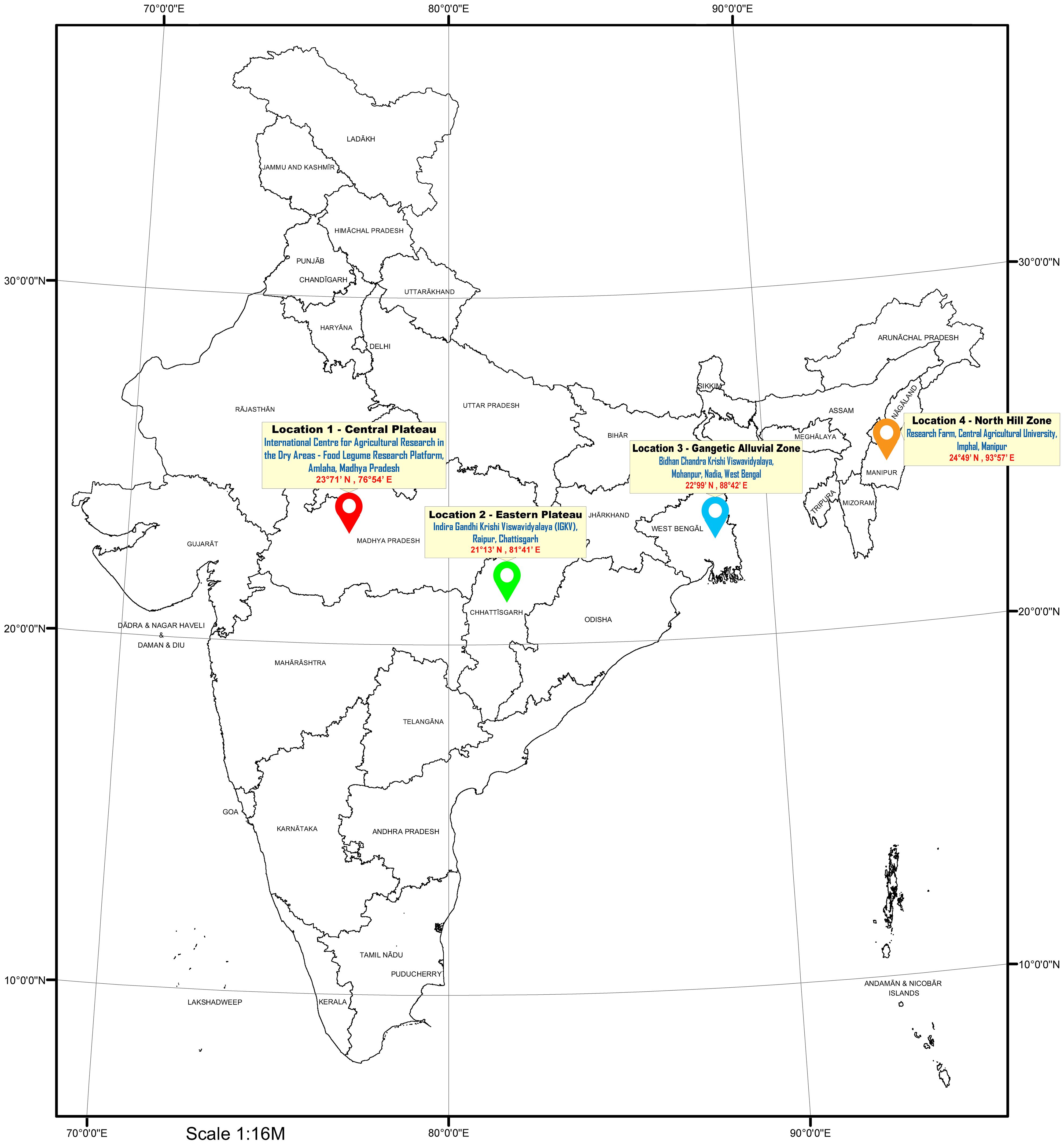
Figure 1. Geographical distribution of the testing locations in different agro-ecological zones in India.

Figure 2

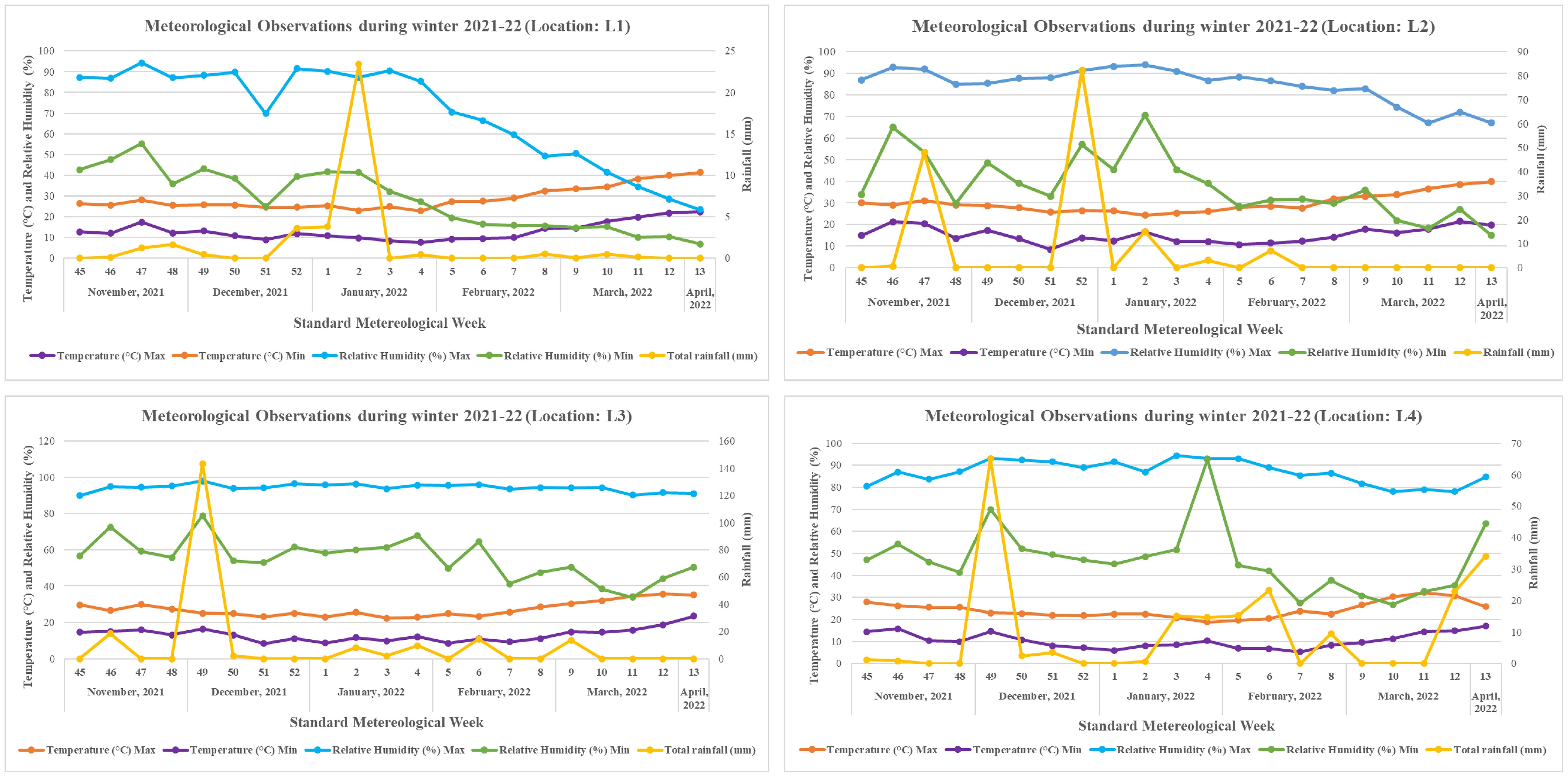
Figure 2. Meteorological observations during winter season of 2021–2022 across the testing locations.

Data analysis and computation of the GGE biplot

Analysis of variance (ANOVA) was computed to reveal the effects of G, E, and GE across the testing locations. The mean significant difference within genotypes and testing locations was calculated using the LSD test at a probability level of p = 0.05. The relatedness of the genotypes and testing locations was represented through hierarchical clustering following the Ward method. In the present study, the Base Linear Phenotypic Selection Index (BLPSI) was enumerated considering the genetic correlation matrix of three important key traits (days to maturity, biological yield, and seed yield) necessary for varietal recommendation of grasspea genotypes. The calculated BLPSI value was plotted as a variable in the GGE biplot to aid in selection regarding the ranking and recommendation of the genotypes as per their general and specific areas of adaptation.

In the GGE biplot model, the main genotypic effect and the GE effects in different test environments were taken into consideration, while the environmental factor was nullified in the evaluation of genotypes (Yan et al., 2000). The biplot was formulated considering the first two principal components (PCs) derived from the singular value decomposition (SVD) of the mean SI. The SVD process decomposed the GGE biplot into eigenvalues of G, SI, and singular values (Yan et al., 2007).

$${\text{Y}}_{\text{ij}}=\text{μ}+{\text{e}}_{\text{j}}+{\displaystyle \sum _{n=1}^N{\lambda }_n}{\text{γ}}_{\text{in}}{\text{δ}}_{\text{jn}}+{\text{ϵ}}_{\text{ij}}$$

Y_ij = yield of the ith grasspea genotypes (i = 1, …, I) in the jth test environments (j = 1, …, J)

µ = grand mean

e_j = environment deviations from the grand mean

λ_n = the eigen value of PC analysis axis

γ_in and δ_jn = genotype and environment PC scores for axis n

N = number of PCs retained in the model

ϵ_ij = error term ~ N (0, σ²)

The current dataset was not subjected to scaling to construct an environment-centered GGE biplot (Yan and Tinker, 2006). The evaluation of genotypes was conducted using genotype-focused singular value partitioning (SVP = 1), while for the testing location evaluation, environment-focused SVP (SVP = 2) was applied (Yan, 2001). The “Average Environment Coordination” (AEC) view of the GGE biplot was created, enabling comparisons of genotypes based on mean SI integrated with stability across environments within a mega-environment (ME), following the approach introduced by Yan (2002). Concomitantly, to assess the test environments, the “discriminating power vs. representativeness” view of the GGE biplot was constructed. The ideal test environment should possess the ability to effectively discriminate among genotypes while also being representative of the ME (Yan et al., 2007). Furthermore, the “which-won-where” view of the GGE biplot was created to facilitate the detection of the superiority of genotypes across the test environments followed by grouping test environments into different MEs based on their performance (Yan and Rajcan, 2002).

Machine learning application

In this study, decision tree-based RF models and artificial neural network-based MLP were utilized for the validation and prediction of different agronomic traits. Both models were chosen for their versatility in handling regression and classification tasks, providing robust predictive capabilities (Hesami et al., 2019; Everingham et al., 2016). RF is a decision tree model that trained multiple trees simultaneously and uses bagging, also known as bootstrap aggregation, for trained trees and showing the final outcome (Pavlov, 2019). The fundamental idea behind the RF model is presented in Equation 1.

$\begin{array}{ll}y={\displaystyle \sum _{i=1}^n({\alpha }_i-{\alpha }_i^{*})}k(x,x_i)+b& (1)\end{array}$

y = observed value of the data point, n = number of samples.

MLP is a feedforward neural network model with three completely interconnected multiple layers of processing nodes in a feedforward manner. Backpropagation is used to train the data until Equation 2 is lowered to update the error-related weights and biases (Katırcı et al., 2021).

$\begin{array}{ll}E=\frac{1}{K}{\displaystyle \sum _{k=1}^K{(y_k-{\widehat{y}}_k)}^2}& (2)\end{array}$

Y = observed value of data point k, k = number of samples.

The leave-one-out cross-validation (LOO-CV) technique that is used for cross-validation was employed in this study (Webb et al., 2011). In LOO-CV, number of folds and instances of data are equal, and learning algorithm is applied to each instance individually. In this way, while using the chosen instance as the single-item test set, all other instances are set as a training set. To find the optimal hyperparameters and building the best model, a grid search approach was used. The open-source Python programming language (Van Rossum and Drake, 2009) was employed for coding with the aid of the sklearn library (Pedregosa et al., 2011). The performance of both models was evaluated by using six performance metrics Equations 3–8, providing insights into their effectiveness and suitability for different applications.

In regression-based ML analysis, regression of coefficient (R²) is the mainstay and exhibits the performance of the model by computing the proportion of variation in the dependent variable. Its value ranges from 0 to 1, and a value close to 1.0 reflects the stronger predictive accuracy of the model.

$\begin{array}{ll}{R}^2=1-\frac{{\displaystyle {\sum }_{i=1}^n}{(Y_i-{\widehat{Y}}_i)}^2}{{\displaystyle {\sum }_{i=1}^n}{(Y_i-\tilde{Y})}^2}& (3)\end{array}$

The root mean square error (RMSE) calculates the prediction errors, and low error scores demonstrate better accuracy of the model.

$\begin{array}{ll}MSE=\sqrt{\frac{1}{n}{\displaystyle \sum _{i=1}^n{(Y_i-{\widehat{Y}}_i)}^2}}& (4)\end{array}$

The average difference between predicted and observed values is measured by the mean absolute error (MAE), and low scores present better accuracy and performance of the model.

$\begin{array}{ll}MAE=\frac{1}{n}{\displaystyle \sum _{i=1}^n|Y_i-{\widehat{Y}}_i|}& (5)\end{array}$

The mean absolute percentage error (MAPE) is the prediction error given in percentage. A high MAPE score reflects a high error and shows the model’s poor performance.

$\begin{array}{ll}MAPE=\frac{1}{n}{\displaystyle \sum _{i=1}^n\left|\frac{Y_i-{\widehat{Y}}_i}{Y_i}\right|\times 100}& (6)\end{array}$

The mean squared logarithmic error (MSLE) is the logarithmic scale of errors and is suitable for datasets with exponential relationships.

$\begin{array}{ll}MSLE=\frac{1}{n}{\displaystyle \sum _{i=1}^n{(\log (Y_i+1)-\log ({\widehat{Y}}_i+1))}^2}& (7)\end{array}$

The median absolute error (MedAE) is based on the median of absolute differences by reducing the effect of outliers in error evaluation.

$\begin{array}{ll}MedAE=median(|Y_1-{\widehat{Y}}_1|,\dots ,|Y_n-{\widehat{Y}}_n|)& (8)\end{array}$

Y_i = measured value; ${\stackrel{⌢}{Y}}_i$ = predicted value; $\overline{Y}$ = measured value’s mean; n = count of samples.

Results

Significance of multilocational trial

ANOVA showcasing the relative contribution of each source of variation to the total variations is presented in Table 1. The ANOVA results indicated that the effects of genotype (G), environment (E), and their interaction (GE) were all found to be statistically significant for all the traits under investigation. Concerning the relative contribution of various components of variation, it was observed that environment has the highest contribution followed by the GE for all the traits under study. The highest contribution of environment was observed for biological yield (86.02%), whereas the contribution of GE was maximum in seed yield (14.98%). The contribution of genotype exhibited the highest effect on seed yield followed by biological yield.

Table 1

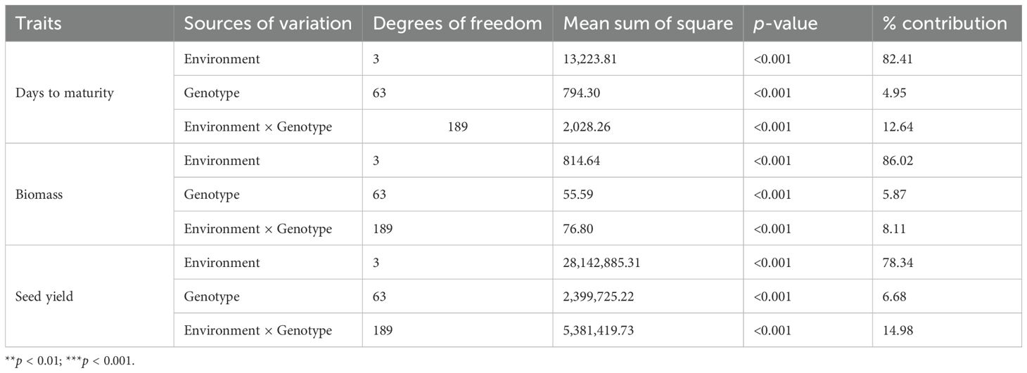
Table 1. Analysis of variance for maturity, biological yield, and seed yield of grasspea genotypes tested across the locations.

Mean performance and descriptive statistics of the grasspea genotypes over the locations

The mean performance of the tested grasspea genotypes considering their maturity, biological yield, and seed yield along with the mean BLPSI is presented in Table 2. Across all locations, FLRP-B54-1-S2 was the early maturity genotype (115 days) with the highest seed yield (1,740.25 kg/ha) potential. The check variety Mahateora matured early along with other six grasspea lines (BANG-147-S3, BANG-234-S1, IGC-2012-4/6-23, BANG-15-S1, IGC-2012-70/1-5, and IGC-2012-31/2-1), although all the genotypes exhibited non-significant differences with each other. Among the locations, genotypes matured early at L2 (106 days) and late in L3 (131 days). Genotypic variance (σ²g) varied between 2.09 (L3) and 6.24 (L4) for the days to maturity trait. Biological yield was significantly highest in genotype 23-GP-F3-S2 (10.51 t/ha) followed by IGC-2012-76/5-14 (9.94 t/ha). Genotypes exhibited the highest biological yield in L2 (11.78 t/ha), which was approximately 52% higher than the average biological yield of the genotypes over the locations. In contrast, L4 (Imphal) exhibited the lowest biological yield (6.09 t/ha), which was approximately 26% lower than the average biological yield of the tested grasspea genotypes over the locations. For this trait, genotypic variance ranged from 0.28 (L1) to 7.45 (L4).

Table 2

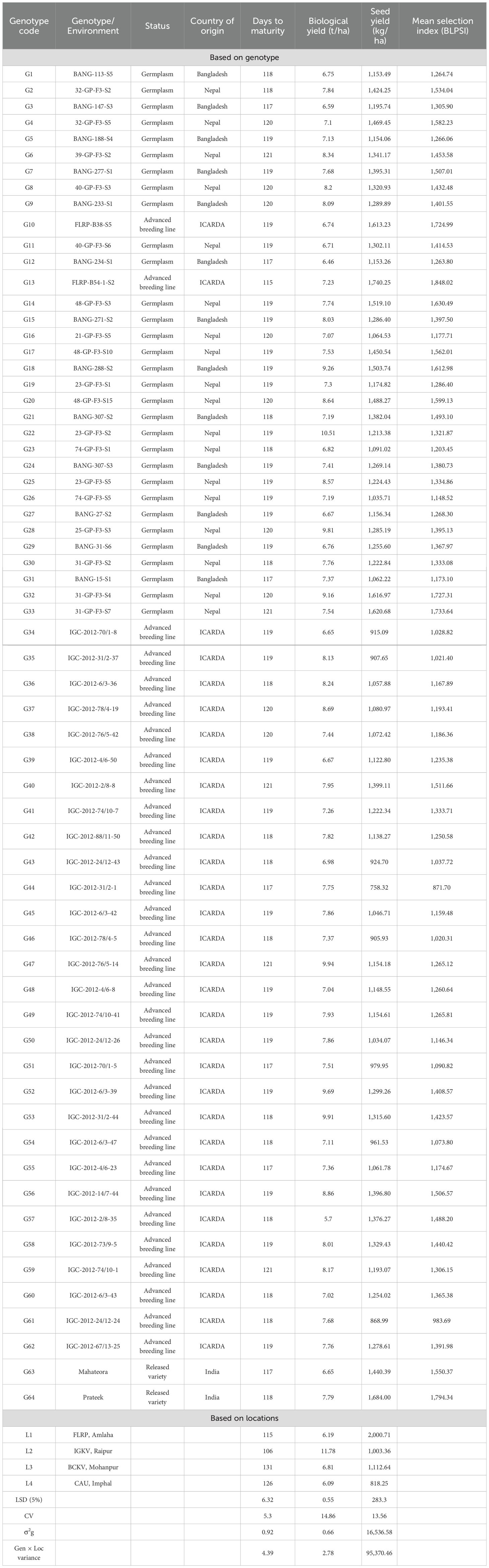
Table 2. Mean performance of the grasspea genotypes across the locations.

Among the check varieties, Prateek recorded the second highest yield (1,684 kg/ha), while maturing within 118 days over the locations. However, non-significant differences were observed between the three promising grasspea genotypes (FLRP-B54-1-S2 > Prateek > 31-GP-F3-S7) concerning yield. All these three genotypes exhibited moderate biological yield ranging from 7.23 to 7.59 t/ha. Among the locations, the highest yield was obtained in L1 (2,000.71 kg/ha), while it was the lowest in L4 (818.25 kg/ha) with a significant difference in the expression of yield potential. The highest genotypic variance as well as GEI was observed for this trait. In the present study, perusal of the data contemplating mean BLPSI reflected that FLRP-B54-1-S2 was detected with having the highest mean BLPSI (1,848.02) among all the tested grasspea genotypes, making it the top-performing genotype considering multi-trait performance. Additionally, Prateek (1,794.34), 31-GP-F3-S7 (1,733.64), 31-GP-F3-S4 (1,727.31), and FLRP-B38-S5 (1,724.99) were also ascertained as good performers considering the mean BLPSI. Among the locations, the highest mean BLPSI was observed in L1 (2,122.22) followed by L3 (1,250.16) with the lowest at L4 (950.01). In L1 (Amlaha), FLRP-B54-1-S2, Prateek, and 31-GP-F3-S7 combined early maturity with high seed yield (>1,600 kg/ha). L2 (Raipur) favored 31-GP-F3-S4, IGC-2012-31/2-44, and 23-GP-F3-S2, which recorded the highest biomass (>9 t/ha). In L3 (Mohanpur), FLRP-B38-S5 and BANG-288-S2 showed a stable seed yield performance (≥1,500 kg/ha), while in L4 (Imphal), IGC-2012-67/13-25 exhibited good adaptability with a superior yield. Overall, FLRP-B54-1-S2, Prateek, 31-GP-F3-S7, and 48-GP-F3-S3 consistently ranked highest across most environments, with seed yield advantages of 8%–15% over the trial mean (Table 2; Figure 3). In the present dataset, it was observed that in L1, out of 64 genotypes, 26 genotypes matured within 105–106 days while 3 genotypes matured beyond 120 days (Figure 3). Interestingly, in L2, maximum genotypic classes were observed and seven genotypes matured within 102 days. In L3, the genotypes matured within the range of 127–133 days while 10 genotypes matured early (127–128 days). In L4, only three classes were obtained, where only 11 genotypes matured within 121 days. In the case of biological yield, in L2, genotypes were divided into five classes, while four classes were observed in the rest of the locations. In contrast, in the case of seed yield, the highest classes were observed in L2 (seven classes) followed by six classes in L4. All the traits exhibited normal distribution over the locations.

Figure 3

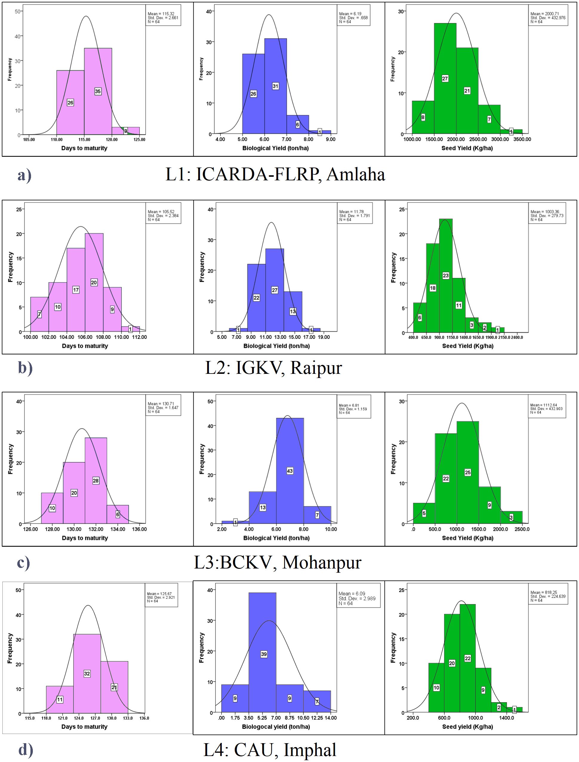
Figure 3. Frequency distribution of yield-attributing traits (days to maturity, biological yield: t/ha; seed yield: kg/ha) in grasspea genotypes over the locations. (a) Frequency distribution of yield-attributing traits in grasspea genotypes at ICARDA-FLRP, Amlaha. (b) Frequency distribution of yield-attributing traits in grasspea genotypes at IGKV, Raipur. (c) Frequency distribution of yield-attributing traits in grasspea genotypes at BCKV, Mohanpur. (d) Frequency distribution of yield-attributing traits in grasspea genotypes CAU, Imphal.

Boxplot analysis represented the distribution of environments concerning three yield components over the locations (Figure 4). For days to maturity, consistent performances were seen in L2. For biological yield and seed yield, a congruous performance was observed in L4 and L1, respectively. In the case of biological yield, L4 and L1 exhibited a stable performance with relatively low variation. Similarly, for seed yield, L4 demonstrated the most uniform performance, suggesting greater consistency in this trait.

Figure 4

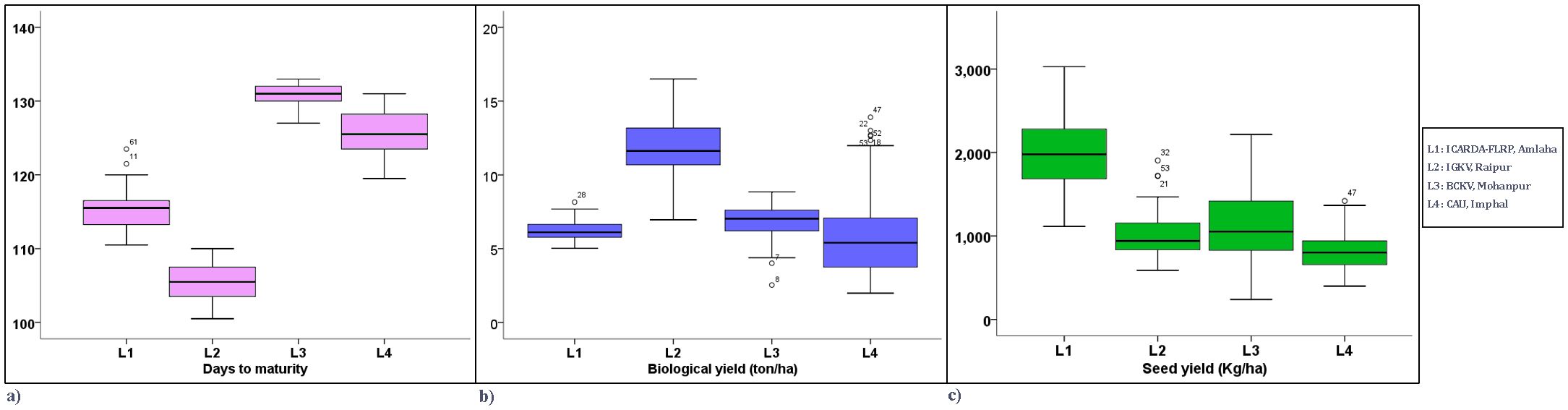
Figure 4. Boxplot view of yield-attributing traits of the grasspea genotypes over the locations. (a) Boxplot view of days to maturity of the grasspea genotypes over the locations. (b) Boxplot view of biological yield (t/ha) of the grasspea genotypes over the locations. (c) Boxplot view of seed yield (kg/ha) of the grasspea genotypes over the locations.

Genetic parameters of the 64 grasspea genotypes for three traits over the locations are presented in Table 3. The mean value for days to maturity was found to be 119 days, and across all the genotypes and locations, the maturity period ranged from 115 to 122 days. In the case of biological trait, moderate variability was observed. Maximum variability was reflected in the case of seed yield and varied between 758 and 1,740 kg/ha. Heritability for maturity (76%) and biological yield (67%) was high, whereas for seed yield, it was moderate (58%).

Table 3

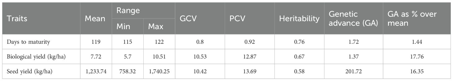
Table 3. Descriptive statistics of the tested grasspea genotypes over the locations.

Genotypic appraisal over the location considering mean vs. stability

The mean performance and stability of the grasspea genotype across different locations considering their mean SI were visually represented using the AEC view of the GGE biplot (Figure 5). In essence, the AEC coordination view of the GGE biplot is a genotype-metric-preserving biplot with an SVP equal to 1. It allows for the visualization of genotype discrimination considering their mean performance. In this graph, the first two PCs enabled to explain 80.93% of the total variation considering mean SI.

Figure 5

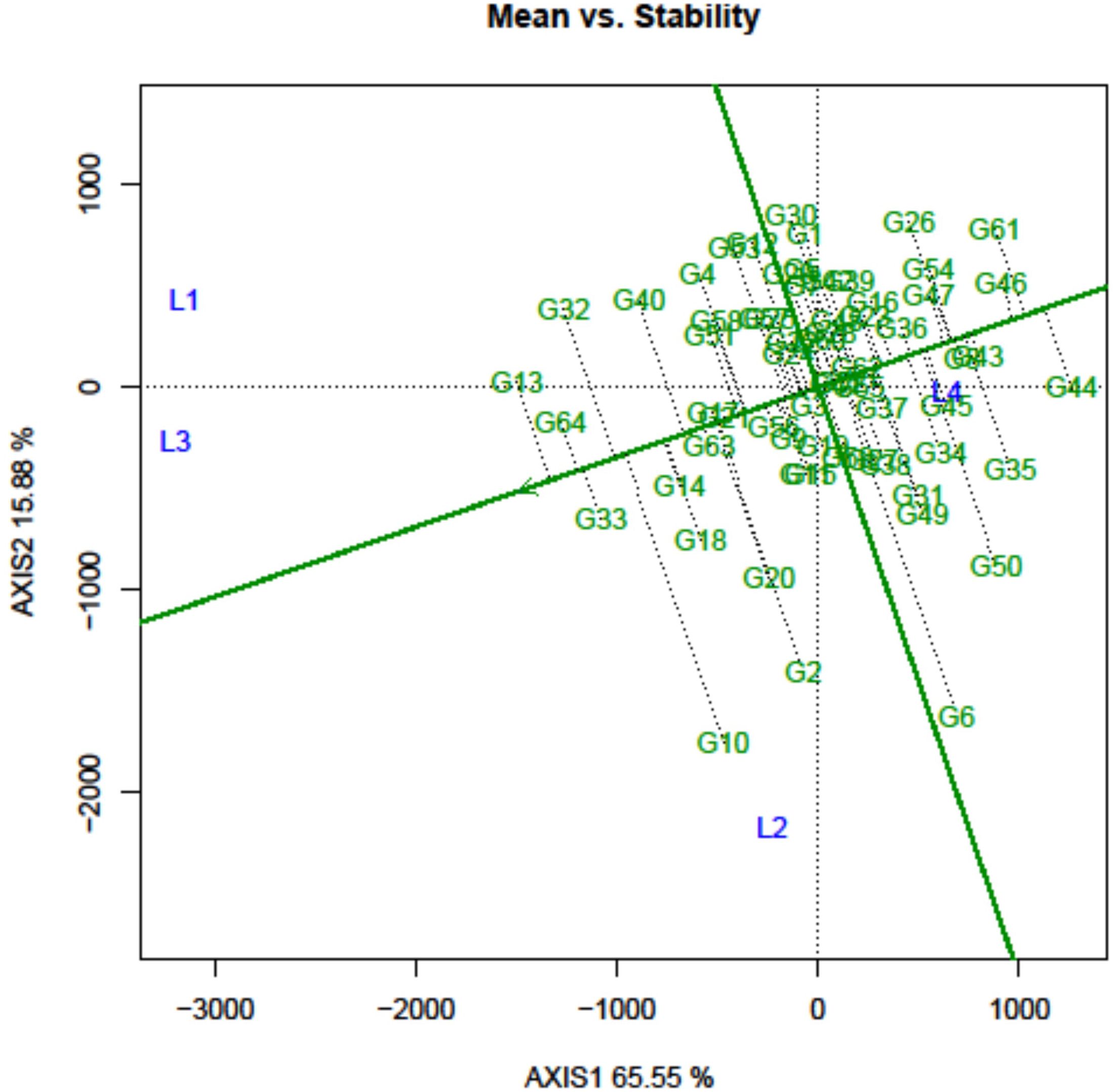
Figure 5. Mean performance and stability of the grasspea genotypes tested across different locations.

The graph’s single arrowhead line represents the AEC abscissa, which passes through the biplot origin and indicates a higher mean SI value of the grasspea genotypes, expressing their overall superiority. The perpendicular line to the AEC, extending outward from the biplot origin, is referred to as the “AEC ordinates”, serving as an indicator of the stability of the genotypes. Inversely, genotypes with longer vector lengths from the AEC abscissa exhibited lower stability, while those with shorter vector lengths were considered more stable. Genotypes FLRP-B54-1-S2 (G13), Prateek (G64), 31-GP-F3-S7 (G33), 31-GP-F3-S4 (G32), FLRP-B38-S5 (G10), 48-GP-F3-S3 (G14), and BANG-288-S2 (G18) exhibited strong multi-trait performance, as they were positioned favorably concerning the “AEC ordinate.” On the other hand, genotypes IGC-2012-31/2-1 (G44), IGC-2012-24/12-24 (G61), and IGC-2012-78/4-5 (G46) performed poorly, as they were positioned in the opposite direction to the “AEC ordinate.” Within the group of good performers, Prateek (G64) and 31-GP-F3-S7 (G33) stood out as the most stable genotypes, as they had shorter projections from the “AEC abscissa.” Despite being the best performer, FLRP-B54-1-S2 (G13) was characterized as an unstable genotype. The present study revealed that Prateek (G64) and 31-GP-F3-S7 (G33) emerged as the most ideal genotypes due to their excellent performance in terms of combined yield-duration profile as well as good stability. The genotypes positioned close to the ideal genotype were regarded as desirable genotypes, and the distance between them is measured using the Euclidean distance. Consequently, 48-GP-F3-S3 (G14) was identified as a desirable genotype because of its proximity to the ideal genotype and nearly stable response in terms of multi-trait performance. Using the mean SI, the tested grasspea genotypes were categorized into seven clusters with promising grasspea genotypes (G13), (G64), (G33), (G32), (G10), (G14), and (G18) in cluster I (Figure 6).

Figure 6

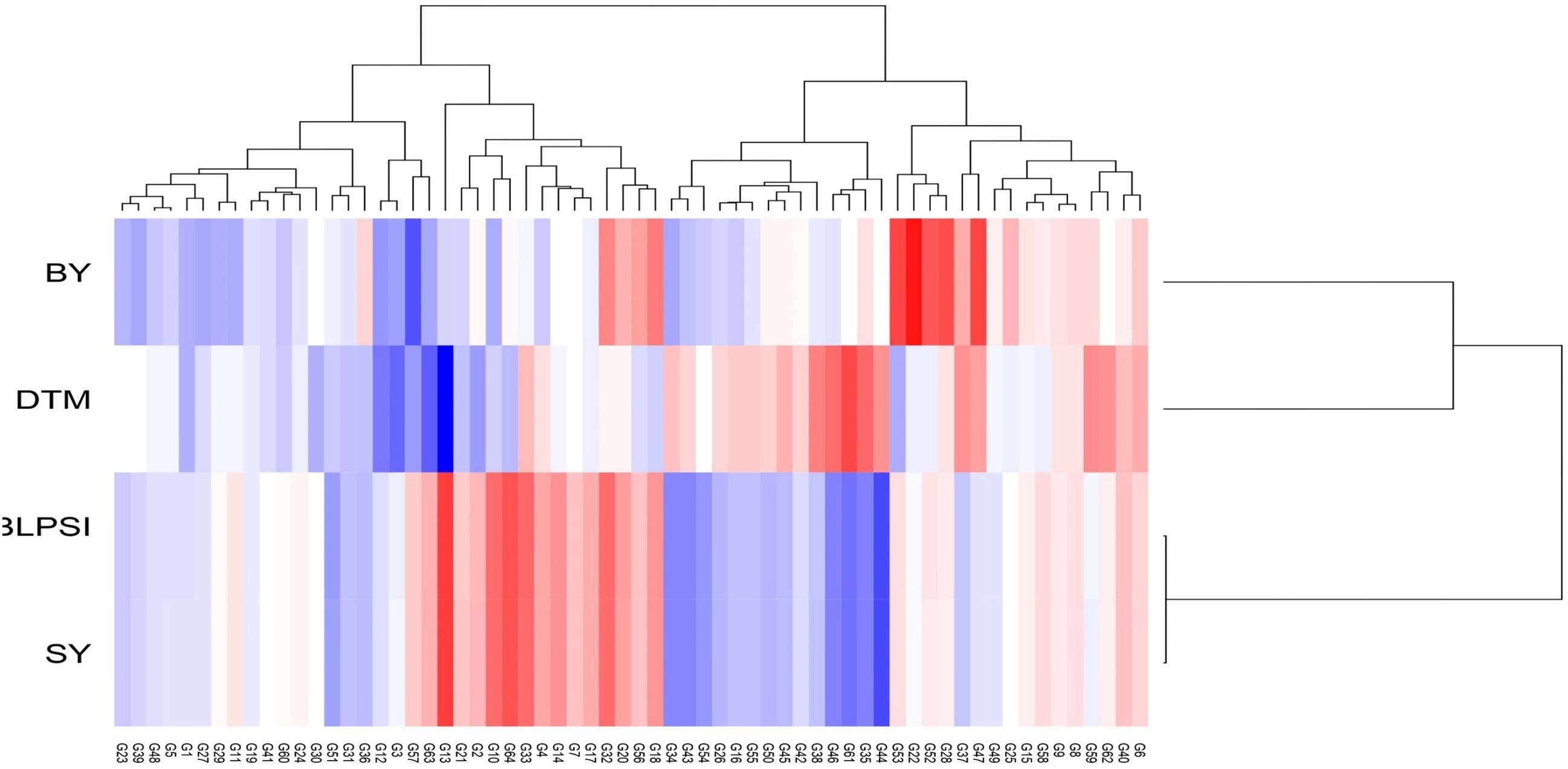
Figure 6. Hierarchical clustering of grasspea genotypes based on days to maturity (DTM), biological yield (BY), seed yield (SY), and the BLPSI over the tested locations.

Environment evaluation following discriminativeness vs. representativeness

In the GGE biplot approach, the critical factors for identifying desirable testing locations and eliminating redundant ones are discrimination power (ability to discriminate genotypes), representativeness (ability to represent corresponding MEs), and the desirability index. In the “discriminativeness vs. representativeness” view of the GGE biplot, the lines connecting the test environments are referred to as environment vectors. From the graph, it was observed that L1 (Amlaha) and L3 (Mohanpur) revealed an acute angle with each other, while the two remaining locations indicated an obtuse angle (Figure 7).

Figure 7

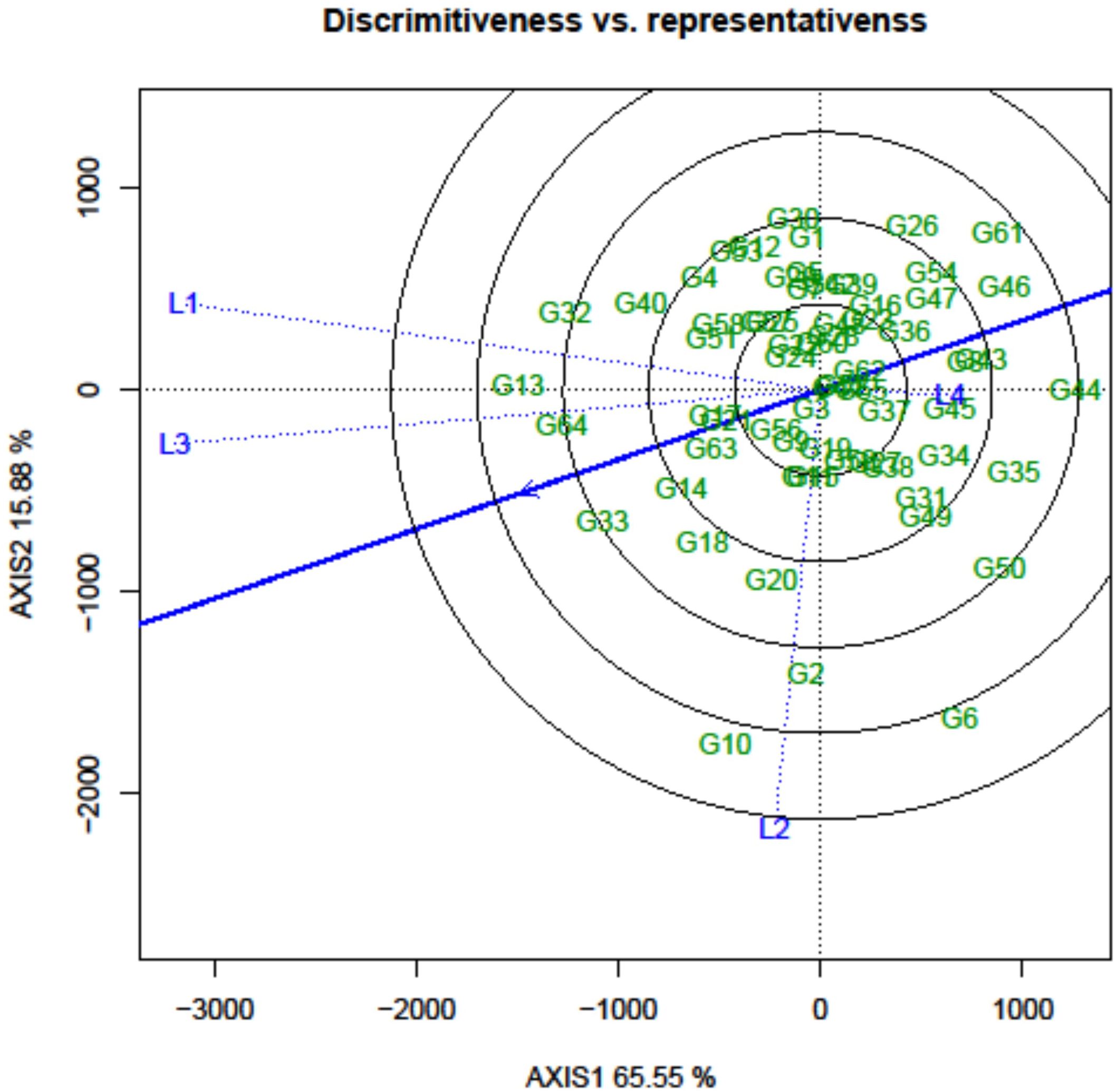
Figure 7. GGE biplot analysis: discriminativeness vs. representativeness of grasspea genotypes tested across different locations.

The information rendered by L4 (Imphal) was distinct from the other locations. Thus, it can be deduced that L1 and L3 environments were positively correlated and had closer relationships with each other. The presence of a close association between these environments suggested that similar information could be obtained regarding genotype performance from these environments.In contrast, an obtuse angle was observed between L1 and L3 on one side and L2 and L4 on the other, indicating a negative association and distant relationships among these environments. The length of the environmental vectors generally represents the discriminating power of the test environments. Therefore, among the four testing locations, L3 (Mohanpur) followed by L1 (Amlaha) were the most discriminative whereas L4 (Imphal) was the least discriminative environment (Table 4).

Table 4

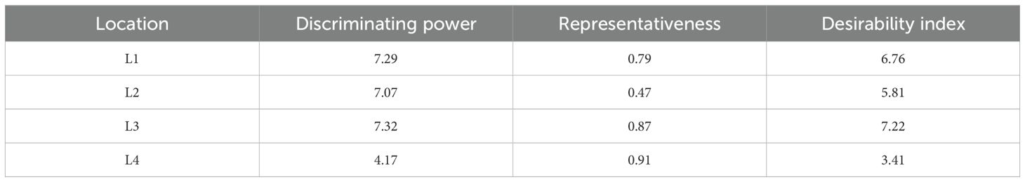
Table 4. Evaluation parameter of the testing environment.

The least discriminative location is also considered as the least informative; thus, this environment can be considered as a redundant testing location for the assessment of grasspea genotypes. The indication of environmental representativeness is typically conveyed by the angle existing between the environment vectors and the AEC. It was observed that L4 (Imphal) reflected with the smallest angle between AEC and was thus identified as the most representative testing location. The desirability index of the test locations encompasses the combined outcome of both discriminative capability and representativeness. L3 (Mohanpur) with the highest desirability index was identified as the ideal testing location for the testing of mini core collection or advance breeding materials as well as for selecting genotypes with general adaptability. However, locations with good discrimination power and less representativeness such as L2 (Raipur) would be meaningful for winnowing genotypes with a specific adaptation. The relatedness of the genotypes and testing locations was represented through hierarchical clustering based on days to maturity, biological yield, and seed yield of the tested grasspea genotypes. All the testing locations were grouped into two clusters (Figure 6).

Delineation of the mega-environment and the winning genotypes

Another crucial aspect of the GGE biplot involves the identification of genotypes suitable for test environments through the graphical depiction known as the “which-won-where” representation. Initially, a polygon was sketched around the genotypes located farthest from the biplot origin, encompassing all the remaining genotypes within its boundaries. Genotypes situated at the polygon’s vertices represent either the most superior or the least favorable performers in one or multiple environments. In the current study, the biplot proved highly informative in effectively distinguishing between environments and displaying a well-distributed polygon (Figure 8). The equality lines divided the graph into seven sectors, with all 4 locations being situated within three of these sectors, which could be designated as “MEs”. The first ME constituted of L1 (Amlaha) and L3 (Mohanpur), and the second and third ME consisted of single location L2 (Raipur) and L4 (Imphal), respectively. The analysis revealed that FLRP-B54-1-S2 (G13) emerged as the winning genotype in ME-I, while in ME-II, FLRP-B38-S5 (G10) was detected as the winning genotype. In the case of ME-III, the genotype positioned in the outer vertex was the poor-performing one; therefore, IGC-2012-67/13-25 (G62) present on the vertex towards the center was considered as the winning genotype.

Figure 8

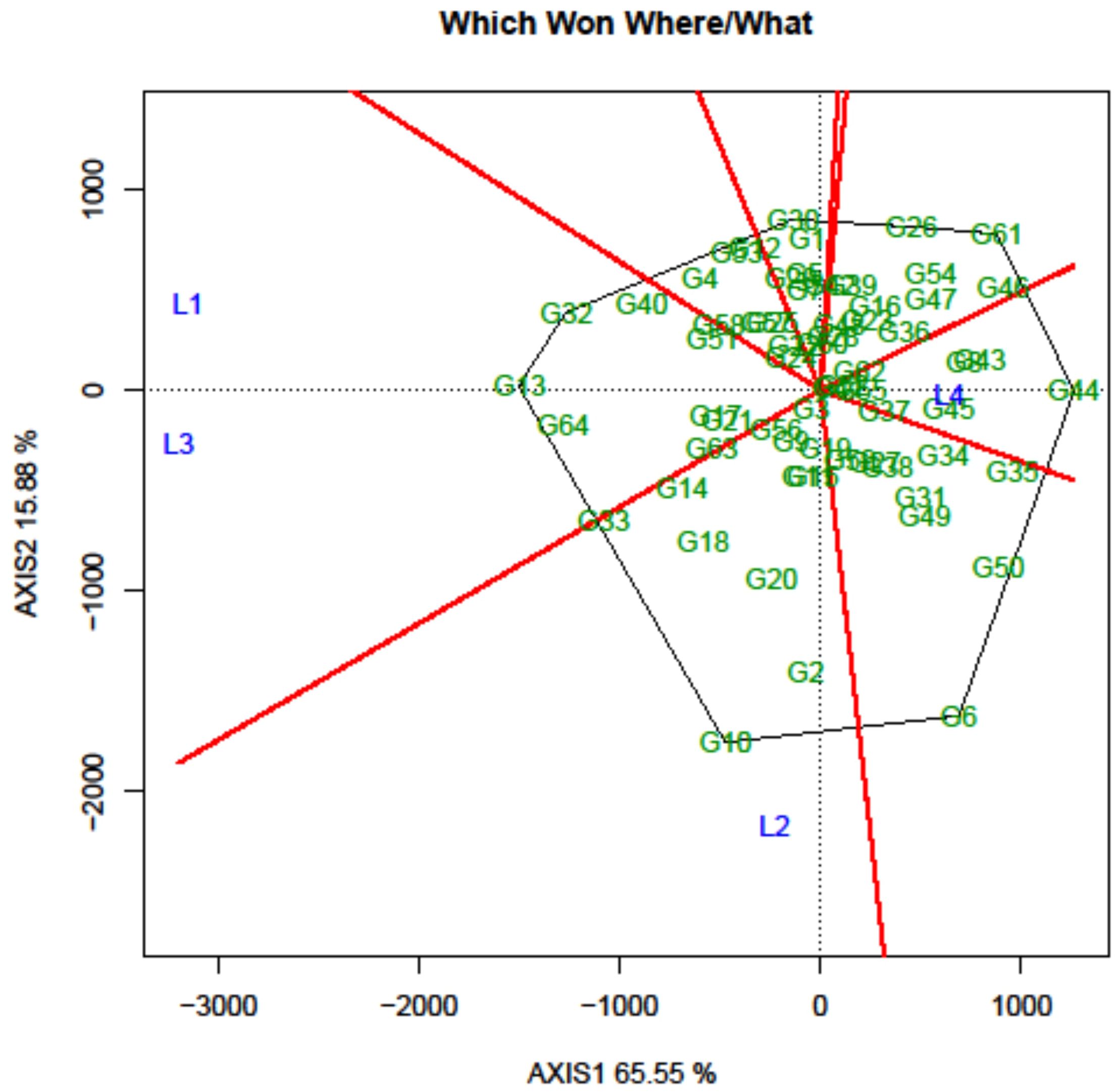
Figure 8. Which-won-where pattern of grasspea genotypes in the GGE biplot analysis tested over the locations.

Machine learning modeling and delimitation of suitable genotypes of grasspea

The present study revealed that the MLP model had the highest R² scores, with values for maturity (MAT) and biological yield (BY) of 0.947 and 0.608, respectively. On the other hand, seed yield (SY) (0.682) and BLPSI (0.679) received the greatest R² values from the RF model (Table 5; Figure 9). These scores indicate the extent to which the independent variables in the model can explain the variance in the dependent variable. Results for MAPE, RMSE, and MLSE were in line with the R² scores, and the lowest scores for MAT and BY from the MLP model demonstrate its superior accuracy and predictive ability. With regard to SY and BLPSI, the RF model performed better as seen by its lower RMSE, MAPE, and MLSE scores. The performance of the MLP model was further validated using the MAE results. The MLP model demonstrated its accuracy in predicting MAT, BY, and SY by achieving the lowest MAE scores for these parameters. The MLSE results showed that both models’ responses to MAT were similar, indicating a similar performance for this metric. For BY, the MLSE score that the MLP model obtained was the lowest. For both SY and BLPSI, the RF model had the lowest MLSE score. The results of the MedAE showed how well the MLP model performed for all parameters.

Table 5

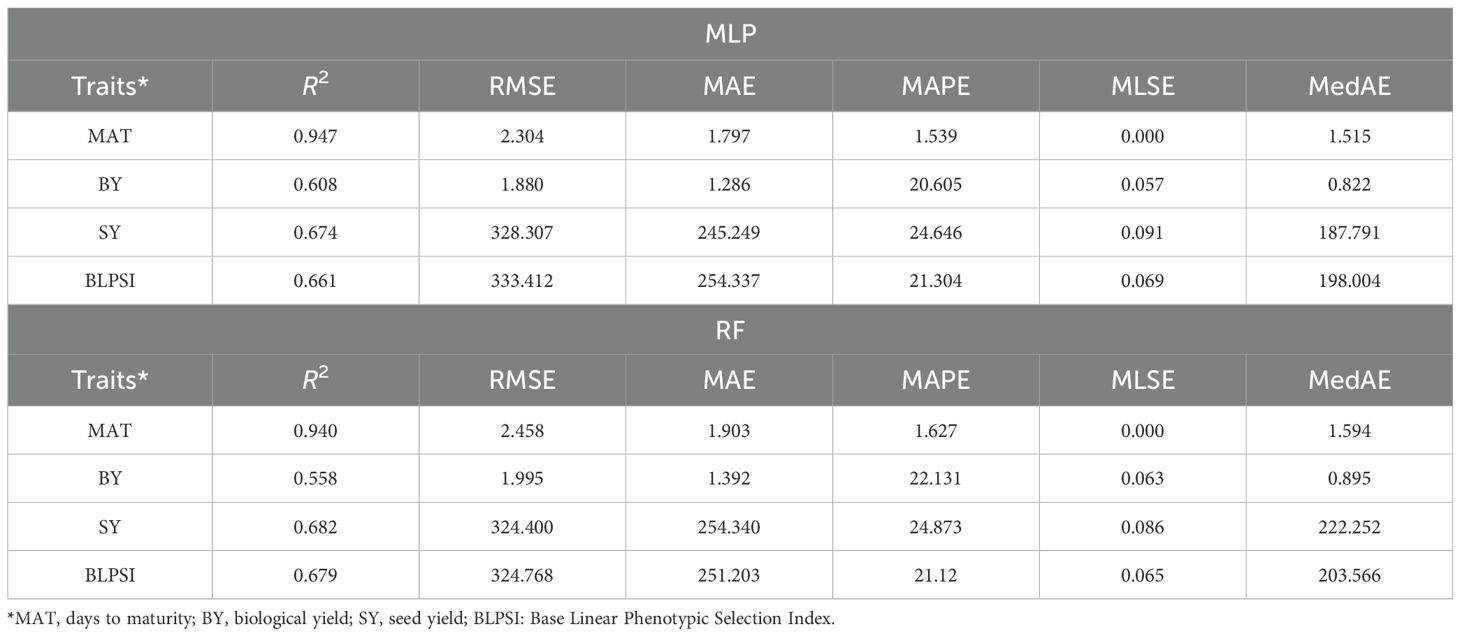
Table 5. Performance metrics of the utilized ML models for different parameters.

Figure 9

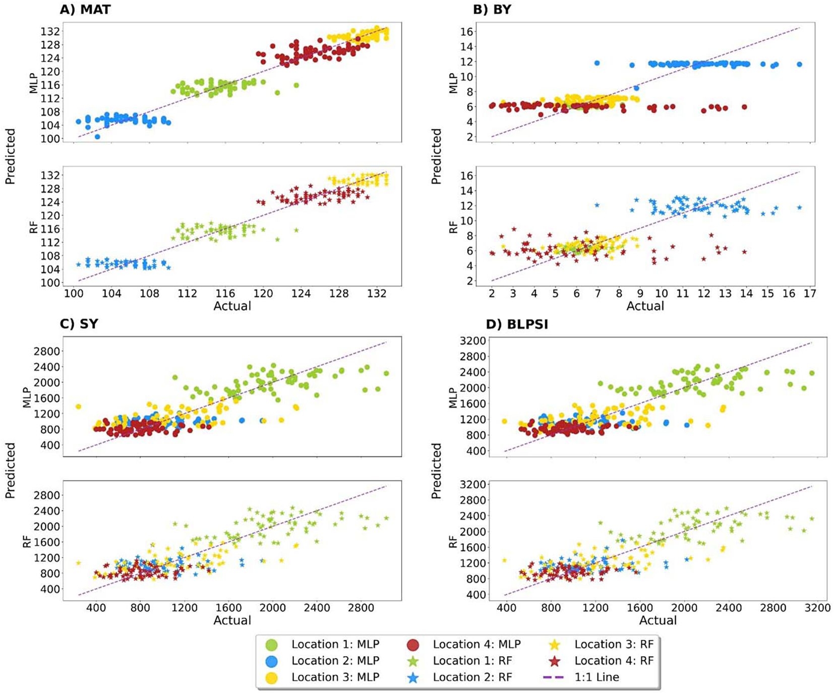
Figure 9. Actual versus predicted scores of grasspea genotypes obtained from the MLP and RF machine learning models across four traits. (A) Performance metrics of the utilized ML models for maturity (MAT), (B) Performance metrics of the utilized ML models for biological yield (BY), (C) Performance metrics of the utilized ML models for seed yield (SY), (D) Performance metrics of the utilized ML models for Base Linear Phenotypic Selection Index (BLPSI).

For all parameters, the MLP model showed lower MedAE values than the RF model, indicating a higher overall predictive accuracy. Overall, the MLP model showed the lowest RMSE, MAPE, MLSE, MAE, and MedAE scores for these parameters, and the highest R² scores for MAT and BY. In contrast, the RF model had the lowest RMSE, MAPE, MLSE, and MAE scores for SY and BLPSI along with the highest R² scores. The MLP model demonstrated exceptional performance in MAE and MedAE, two crucial metrics for evaluating prediction accuracy and resilience.

Discussion

Plant breeders frequently conduct multi-location trials (MLTs) to assess the test entries. This practice forms a strong foundation for the adoption and commercial release of varieties. Grasspea is a versatile crop concerning its wide adaptability (Das et al., 2021). The testing locations in the present study represent the diverse agro-climatic zones in India. In multi-locational trials, the variance components are mainly divided into three classes, main effect of genotype, environment, and their interaction (GE). The presence of the GE component adds ambiguity to genotype evaluation due to inconsistency in the performance of cultivars across different locations. Understanding the GEI is crucial for refining breeding strategies, selecting non-redundant testing sites, and recommending varieties for specific or broad adaptation. Over the past decade, Additive Main Effect and Multiplicative Interaction (AMMI) (Ahmadi et al., 2012; Rajendran et al., 2018; Rubiales et al., 2020) and the GGE biplot (Yan et al., 2007; Chatterjee et al., 2019) have gained prominence for the visual representation of GEIs, facilitating the identification of stable genotypes and optimal environments. The GGE biplot surpasses AMMI in ME analysis through elucidating a greater proportion of G+GE and providing insights into optimizing test environments through the “discrimination power vs. representativeness” graph (Yan et al., 2007). The present study attempted to cull out stable grasspea genotypes with a minimal GEI impact and a greater genetic buffering capacity employing the GGE biplot methodology.

In the present study, ANOVA confirmed the significant contributions of the environment and GEI for all the studied traits, which were considered for estimating the mean BLPSI, thereby corroborating the relevance of MLTs. Earlier literature (Gauch and Zobel, 1997) suggested that, in MLT data, the primary source of variation is the environment, accounting for over 80% of the total variation. In mungbean (Das et al., 2020; Singh et al., 2020), fieldpea (Das et al., 2019; Biswas et al., 2021), chickpea (Tamang et al., 2021), and lentil (Bhattacharya et al., 2022a, 2022b; Chatterjee et al., 2023), studies aligned with the current results, highlighting the prominence of environmental variation. In the current investigation, the substantial contribution of GEI was also evident, underscoring the presence of distinct MEs within the tested locations (Gore et al., 2021).

In MLTs, breeders must recommend genotypes based on combined yield-trait performance. However, most studies focus on single trait analysis, leaving other traits unexplored (Yan and Tinker, 2006). To address this, decisions must be taken considering the breeder’s experience and judgment for framing a selection index or subjective weight for multiple traits. In the present study, we have tried to visualize the GEI effect based on combined multi-trait performance of the grasspea genotypes wherein beside yield performance, maturity and biomass were also taken into consideration. It was observed that the performance of grasspea genotypes was unpredictable and inconsistent at different locations and ratified the presence of crossover interaction (COI). Genotypes G13, G33, G10, G63, and G6 showed promise in L1, while in L2, G32, G53, G21, G4, and G50 excelled. The presence of COI implied breeding for specific adaptation (Yan and Hunt, 2002; Rakshit et al., 2012). However, some genotypes (G13 and G33) exhibited non-COI, aligning with previous studies showing the presence of both COI and non-COI within the same datasets (Das et al., 2019; Singh et al., 2020). This complexity may diminish the genetic gain due to the intricacies during the selection procedure (Comstock and Moll, 1963).

The GGE biplot simplifies the complex interaction between the genotype, environment, and GEI in the form of different PCs, and their contribution justifies the usefulness of the methodology for explaining the sources of variation (Yan and Tinker, 2005). In this study, the two PCs explained more than 80% of the variation, which rationalized the adequacy of the MLT in grasspea. The ideal genotype selection in the GGE biplot is based on both mean performance and stability. In the present study, Prateek (G64) and 31-GP-F3-S7 (G33) were considered as the ideal genotypes due to their high BLPSI value considering multi-trait performance and minimal interaction with the environment in the form of less projection from “the AEC abscissa” (Yan and Falk, 2002). Genotypes that are close to the “ideal” genotypes are considered as “desirable” genotypes due to having their high genetic relationship with the “ideal” genotype (Yan and Tinker, 2005). 48-GP-F3-S3 (G14) was identified as a desirable genotype due to its close positional proximity with the ideal genotype. Genotype positioning along the AEC ordinate indicated performance variation across environments, likely influenced by weather parameters such as rainfall, temperature, and humidity (Dehghani et al., 2006). Thus, genotypes with low homeostasis exhibit high responsiveness towards environments.

Another important feature of the GGE biplot is the culling out of the optimal testing location judiciously with an aim of efficiently distributing resources, while also minimizing the overall trial costs. Importantly, this allocation strategy was designed to ensure that trial heritability and genetic gain under selection were not compromised in the process (Yan, 2001). Within the GGE framework, the projection of the vector onto the “AEC abscissa” plays a pivotal role in determining both the overall impact of the environment and the effectiveness of the methodology employed (Allen, 1978; Flores et al., 2013). In legume crops such as grasspea, where the additive component of variation holds a dominant role, the vector projection of the testing location on the GGE biplot serves as an indirect selection parameter, which is instrumental in confirming the effectiveness of the methodology being used (Yan and Holland, 2010). Taking all factors into account, L3 (Mohanpur) emerged as the optimal testing location due to its highest desirability index, being both discriminative and representative of the target environments. This selection makes it the ideal choice for evaluating advanced breeding materials, especially with a meager seed quantity that needs to be adjusted across various locations.

Additionally, the GGE biplot was able to separate all the testing locations into three MEs to aid the restructuring of agro-ecological zonation with the winning genotype for each center. An ME can be defined as a group of analogous locations delivering a similar genotypic response and sharing the same set of genotypes across the year (Yan and Rajcan, 2002). The “ideal” genotype identified in the present study, G13 (FLRP-B54-1-S2), was also the winning genotype in ME-I, while FLRP-B38-S5 (G10) for ME-II and IGC-2012-67/13-25 (G62) in ME-III revealed specific adaptation for the respective MEs. Prior research has utilized the GGE approach to assess testing locations and delineate specific environmental zones in a similar manner (Sayar and Han, 2015; Chatterjee et al., 2019; Vaezi et al., 2023).

The application of ML models in this study provided deeper insights into GEIs, improving predictive accuracy for key yield traits. The MLP model, with its ability to capture nonlinear relationships, performed well in predicting maturity and biological yield, benefiting from automated feature learning and multicollinearity handling (Sarker, 2021; Akay et al., 2022). Its strength in modeling continuous variables contributed to improved accuracy, particularly for traits influenced by multiple factors. Comparable integrative approaches using the GGE biplot and ML have been reported in cereals, providing useful benchmarks for our findings. For instance, Omrani et al. (2025) applied RF and MLP models alongside GGE analysis in wheat and found that combining multi-trait indices with predictive modeling improved genotype ranking stability compared to single-trait models, which is consistent with our observation that ML integration better captured genotype × environment patterns in grasspea.

Conversely, the RF model proved more effective in handling high-dimensional data, particularly for seed yield and soil-related traits (Wani et al., 2022). Its ensemble averaging approach reduced sensitivity to noise and outliers, resulting in more stable predictions. Additionally, its ability to rank feature importance provided valuable insights into the most influential agronomic factors (Fawagreh et al., 2014). The integration of ML with the GGE biplot approach further improved genotype selection for the Indian climate. ML models identified complex genotype × environment patterns, facilitating the selection of high-yielding and climate-adapted grasspea genotypes (Bello et al., 2015). This data-driven approach enhanced selection efficiency, making trait evaluation more precise and supporting climate-resilient breeding strategies.

The observed performance differences between MLP and RF highlight the importance of model selection based on trait characteristics. While MLP was effective for complex, continuous traits, RF provided robustness in high-dimensional datasets, making it particularly useful for trait selection and stability analysis. These findings emphasize the role of ML in improving prediction accuracy and decision-making in crop improvement programs. Thus, AI-driven tools can efficiently model and visualize these interactions, enabling researchers to identify genotypes with superior adaptability and yield potential in varied Indian climates. This approach makes data-driven decisions in genotype selection and breeding strategies, improving the efficiency and accuracy of identifying suitable grasspea genotypes.

Conclusion

The present study highlighted the significant environmental and genotype × environment effects on grasspea performance across diverse Indian locations. GGE biplot analysis grouped the sites into three MEs, identifying FLRP-B54-1-S2, Prateek, and 31-GP-F3-S7 as ideal genotypes, and 48-GP-F3-S3 as a desirable genotype for targeted adaptation. ML models complemented traditional analyses, with MLP performing best for maturity and biomass, and RF for seed yield and BLPSI. This synergistic data-driven approach for genotype selection and identifying the ideal test environment can strengthen the substantial selection of location with optimization of resources in future breeding programs.

Data availability statement

The original contributions presented in the study are included in the article/Supplementary Material. Further inquiries can be directed to the corresponding authors.

Author contributions

SBa: Conceptualization, Data curation, Formal analysis, Methodology, Writing – original draft, Writing – review & editing. AD: Data curation, Formal analysis, Writing – original draft. MP: Data curation, Writing – review & editing. SY: Data curation, Writing – review & editing. MA: Formal analysis, Methodology, Software, Writing – review & editing. SA: Formal analysis, Software, Writing – review & editing, Methodology. AS: Writing – review & editing. AY: Formal analysis, Writing – review & editing. ND: Writing – review & editing. SKa: Writing – review & editing. SBh: Data curation, Writing – review & editing. SR: Writing – review & editing, Data curation. SG: Writing – review & editing. SKu: Conceptualization, Funding acquisition, Project administration, Supervision, Writing – review & editing.

Funding

The author(s) declare financial support was received for the research and/or publication of this article. This work has funding support from the International Center for Agricultural Research in the Dry Areas (ICARDA), India.

Conflict of interest

The authors declare that the research was conducted in the absence of any commercial or financial relationships that could be construed as a potential conflict of interest.

Generative AI statement

The author(s) declare that no Generative AI was used in the creation of this manuscript.

Any alternative text (alt text) provided alongside figures in this article has been generated by Frontiers with the support of artificial intelligence and reasonable efforts have been made to ensure accuracy, including review by the authors wherever possible. If you identify any issues, please contact us.

Publisher’s note

All claims expressed in this article are solely those of the authors and do not necessarily represent those of their affiliated organizations, or those of the publisher, the editors and the reviewers. Any product that may be evaluated in this article, or claim that may be made by its manufacturer, is not guaranteed or endorsed by the publisher.

Supplementary material

The Supplementary Material for this article can be found online at: https://www.frontiersin.org/articles/10.3389/fpls.2025.1647903/full#supplementary-material

References

Aasim, M., Ali, S. A., Altaf, M. T., Ali, A., Nadeem, M. A., and Baloch, F. S. (2023). Artificial neural network and decision tree facilitated prediction and validation of cytokinin-auxin induced in vitro organogenesis of sorghum (Sorghum bicolor L.). Plant Cell Tissue Organ Culture (PCTOC) 153, 611–624. doi: 10.1007/s11240-023-02498-3

Crossref Full Text | Google Scholar

Ahmadi, J., Vaezi, B., Shaabani, A., and Khademi, K. (2012). Multi-environment yield trials of grass pea (Lathyrus sativus L.) in Iran using AMMI and SREG GGE. J. Agr. Sci. Tech. 14, 1075–1085.

Google Scholar

Akay, B., Karaboga, D., and Akay, R. (2022). A comprehensive survey on optimizing deep learning models by metaheuristics. Artif. Intell. Rev. 55, 829–894. doi: 10.1007/s10462-021-09992-0

Crossref Full Text | Google Scholar

Allen, F. L. (1978). Comstock RE, Rasmusson DC. Optimal environments for your testing. Crop Sci. 18, 747–751. doi: 10.2135/cropsci1978.0011183X001800050013x

Crossref Full Text | Google Scholar

Almeida, R. D. C., Neto, W. V. D. A., Silva, V. B. D., Carvalho, L. C. B., Lopes, Â.C.D.A., and Gomes, R. L. F. (2021). Decision tree as a tool in the classification of lima bean accessions. Rev. Caatinga 34, 471–478. doi: 10.1590/1983-21252021v34n223rc

Crossref Full Text | Google Scholar

Banerjee, J., Das, A., Parihar, A. K., Sharma, R., Pramanik, K., and Barpete, S. (2022). “Genomic designing towards development of abiotic stress tolerant grass pea for food and nutritional security,” in Genomic Designing for Abiotic Stress Resistant Pulse Crops (Springer International Publishing, Cham), 345–381.

Google Scholar

Barbosa, A., Trevisan, R., Hovakimyan, N., and Martin, N. F. (2020). Modeling yield response to crop management using convolutional neural networks. Comput. Electron. Agric. 170, 105197. doi: 10.1016/j.compag.2019.105197

Crossref Full Text | Google Scholar

Barpete, S., Altaf, M. T., Liaqat, W., Ali, A., Bedir, M., Nadeem, M. A., et al. (2025). “Application of next-generation breeding tools in minor pulses for major impact: A way ahead,” in Breeding Climate Resilient and Future Ready Pulse Crops (Singapore: Springer), 317–350. doi: 10.1007/978-981-96-0483-8_11

Crossref Full Text | Google Scholar

Barpete, S., Chatterjee, S., Roy, S., Murmu, M., Dutta, P., Das, A., et al. (2024). Biotic stresses in grasspea: status and outlook of genomics-aided breeding strategies. Genomics-aided Breed. Strategies Biotic Stress Grain Legumes 14, 405–441. doi: 10.1007/978-981-97-3917-2_12

Crossref Full Text | Google Scholar

Barpete, S., Das, A., Kahriz, P. P., Kahriz, M. P., Khawar, K. M., Qunale, X., et al. (2023). Disease resistance breeding in lathyrus sativus L. Diseases in legume crops: next generation breeding approaches for resistant legume crops Diseases in Legume Crops 26, 233–256. doi: 10.1007/978-981-99-3358-7

Crossref Full Text | Google Scholar

Bello, O., Holzmann, J., Yaqoob, T., and Teodoriu, C. (2015). Application of artificial intelligence methods in drilling system design and operations: a review of the state of the art. J. Artif. Intell. Soft. Computing Res. 5, 121–139. doi: 10.1515/jaiscr-2015-0024

Crossref Full Text | Google Scholar

Bhattacharya, S., Das, A., Banerjee, J., Mandal, S. N., Kumar, S., and Gupta, S. (2022a). Elucidating genetic variability and genotype × environment interactions for grain iron and zinc content among diverse genotypes of lentil (Lens culinaris). Plant Breed. 141, 786–800. doi: 10.1111/pbr.13053

Crossref Full Text | Google Scholar

Bhattacharya, S., Das, A., Banerjee, J., Mandal, S., and Mandal, G. S. (2022b). Delineation of stable high yielding lentil genotypes through HA-GGE and REML/BLUP method for gangetic alluvial zone of India. Leg Res. doi: 10.18805/LR-4928

Crossref Full Text | Google Scholar

Biswas, T., Mazumdar, D., Das, A., Kumar, P. D., Maji, A., Parihar, A. K., et al. (2021). Additive main effects and multiplicative interactions in field pea (Pisum sativum L.) genotypes across the major agro-climatic zones in India. Legume Res. 44, 894–899. doi: 10.18805/LR-4166.

Crossref Full Text | Google Scholar

Chatterjee, S., Das, A., Bhattacharya, S., Banerjee, J., Gupta, S., and Kumar, S. (2023). Identification of suitable genotypes of lentil (Lens culinaris) for improved adaptation to rice fallow areas of Gangetic Alluvial Zone. Indian J. Agric. Sci. 93, 862–867. doi: 10.56093/ijas.v93i8.125345

Crossref Full Text | Google Scholar

Chatterjee, C., Debnath, M., Karmakar, N., and Sadhukhan, R. (2019). Stability of grass pea (Lathyrus sativus L.) genotypes in different agroclimatic zone in eastern part of India with special reference to West Bengal. Genet. Resour. Crop Evol. 66, 1515–1531. doi: 10.1007/s10722-019-00809-2

Crossref Full Text | Google Scholar

Comstock, R. E. and Moll, R. H. (1963). “Genotype—environment interactions: analysis and problems. In: Quantitative and Ecological Aspects of Plant Breeding (Dordrecht: Springer). doi: 10.1007/978-94-011-5830-5_6

Crossref Full Text | Google Scholar

Das, A., Gupta, S., Parihar, A. K., Singh, D., Chand, R., Pratap, A., et al. (2020). Delineating Genotype× Environment interactions towards durable resistance in mungbean against Cercospora leaf spot (Cercospora canescens) using GGE biplot. Plant Breed. 139, 639–650. doi: 10.1111/pbr.12789

Crossref Full Text | Google Scholar

Das, A., Parihar, A. K., Barpete, S., Kumar, S., and Gupta, S. (2021). Current perspectives on reducing the β-ODAP content and improving potential agronomic traits in grass pea (Lathyrus sativus L.). Front. Plant Sci. 12, 703275. doi: 10.3389/fpls.2021.703275

PubMed Abstract | Crossref Full Text | Google Scholar

Das, A., Parihar, A. K., Saxena, D., Singh, D., Singha, K. D., and Kushwaha, K. P. S. (2019). Deciphering genotype-by-environment interaction for targeting test environments and rust resistant genotypes in field pea (Pisum sativum L.). Front. Plant Sci. 10, 825. doi: 10.3389/fpls.2019.00825

PubMed Abstract | Crossref Full Text | Google Scholar

Dehghani, H., Ebadi, A., and Yousefi, A. (2006). Biplot analysis of genotype by environment interaction for barley yield in Iran. Agron. J. 98, 388–393. doi: 10.2134/agronj2004.0310

Crossref Full Text | Google Scholar

Everingham, Y., Sexton, J., Skocaj, D., and Inman-Bamber, G. (2016). Accurate prediction of sugarcane yield using a random forest algorithm. Agron. Sustain. Dev. 36, 1–9. doi: 10.1007/s13593-016-0364-z

Crossref Full Text | Google Scholar

Fawagreh, K., Gaber, M. M., and Elyan, E. (2014). Random forests: from early developments to recent advancements. Syst. Sci. Control Engineering: Open Access J. 2, 602–609. doi: 10.1080/21642583.2014.956265

Crossref Full Text | Google Scholar

Flores, F., Hybl, M., Knudsen, J. C., Marget, P., Muel, F., Nadal, S., et al. (2013). Adaptation of spring faba bean types across European climates. Field Crops Res. 145, 1–9. doi: 10.1016/j.fcr.2013.01.022

Crossref Full Text | Google Scholar

Gauch, H. G., Jr. and Zobel, R. W. (1997). Identifying mega-environments and targeting genotypes. Crop Sci. 37, 311–326. doi: 10.2135/cropsci1997.0011183X003700020002x

Crossref Full Text | Google Scholar

Gore, P. G., Das, A., Bhardwaj, R., Tripathi, K., Pratap, A., and Dikshit, H. K. (2021). Understanding G × E interaction for nutritional and antinutritional factors in a diverse panel of Vigna stipulacea (Lam.) Kuntz germplasm tested over the locations. Front. Plant Sci. 12, 766645. doi: 10.3389/fpls.2021.766645

PubMed Abstract | Crossref Full Text | Google Scholar

Hair, J. F., Black, W. C., Babin, B. J., and Anderson, R. E. (2019). Multivariate data analysis. 8th ed (Boston: Cengage).

Google Scholar

Hamdia, K. M., Zhuang, X., and Rabczuk, T. (2021). An efficient optimization approach for designing machine learning models based on genetic algorithm. Neural Computing Appl. 33, 1923–1933. doi: 10.1007/s00521-020-05035-x

Crossref Full Text | Google Scholar

Hesami, M., Naderi, R., and Tohidfar, M. (2019). Modeling and optimizing in vitro sterilization of chrysanthemum via multilayer perceptron-non-dominated sorting genetic algorithm-II (MLP-NSGAII). Front. Plant Sci. 10, 282. doi: 10.3389/fpls.2019.00282

PubMed Abstract | Crossref Full Text | Google Scholar

Katırcı, R., Yılmaz, E. K., Kaynar, O., and Zontul, M. (2021). Automated evaluation of Cr-III coated parts using mask RCNN and ML methods. Surf Coat Technol 422, 127571.

Google Scholar

Khanal, S., Zhang, H., and Taeihagh, A. (2024). Development of new generation of artificial intelligence in China: when Beijing’s global ambitions meet local realities. J. Contemp. China, 1–24. doi: 10.1080/10670564.2024.2333492

Crossref Full Text | Google Scholar

Kumar, S., Gupta, P., Barpete, S., Choukri, H., Maalouf, F., and Sarkar, A. (2021). “Grass pea,” in The Beans and the Peas, From Orphan to Mainstream Crops. Eds. Pratap, A. and Gupta., S. (Woodhead Publishing), 273–287. doi: 10.1016/B978-0-12-821450-3.00005-6

Crossref Full Text | Google Scholar

Lambein, F. (2000). Homeopathy, longevity and Lathyrus sativus toxicity. Lath Lath Newsl. 1, 4–5.

Google Scholar

Mahapatra, N. S., Das, A., Bhattacharyya, P., Bhattacharya, S., Pal, S., and Barpete, S. (2020). Studies on genetic variability, divergence and association of characters in grass pea. J. Crop Weed 16, 155–161. doi: 10.22271/09746315.2020.v16.i1.1287

Crossref Full Text | Google Scholar

Najafabadi, M. M., Villanustre, F., Khoshgoftaar, T. M., Seliya, N., Wald, R., and Muharemagic, E. (2015). Deep learning applications and challenges in big data analytics. J. Big Data 2, 1–21. doi: 10.1186/s40537-014-0007-7

Crossref Full Text | Google Scholar

Ninomiya, S. (2022). High-throughput field crop phenotyping: current status and challenges. Breed. Sci. 72, 3–18. doi: 10.1270/jsbbs.21069

PubMed Abstract | Crossref Full Text | Google Scholar

Nogueira, E., Oliveira, B., Bulcão-Neto, R., and Soares, F. (2023). A systematic review of the literature on machine learning methods applied to high throughput phenotyping in agricultural production. IEEE Latin America Trans. 21, 783–796. doi: 10.1109/TLA.2023.10244177

Crossref Full Text | Google Scholar

Omrani, A., Omrani, S., Shojaei, S. H., Holasou, H. A., Türkoğlu, A., and Afzalifar, A. (2025). Analysing wheat productivity: using GGE biplot and machine learning to understand agronomic traits and yield. Cereal Res. Commun. doi: 10.1007/s42976-024-00615-2

Crossref Full Text | Google Scholar

Osco, L., Junior, J., Ramos, A., Furuya, D., Santana, D., Teodoro, L., et al. (2020). Leaf nitrogen concentration and plant height prediction for maize using UAV-based multispectral imagery and machine learning techniques. Remote Sens. 12, 3237. doi: 10.3390/rs12193237

Crossref Full Text | Google Scholar

Osco, L. P., Ramos, A. P. M., Pereira, D. R., Moriya, A. S., Imai, N. N., Matsubara, E. T., et al. (2019). Predicting canopy nitrogen content in citrus-trees using random forest algorithm associated to spectral vegetation indices from UAV-imagery. Remote Sens. 11, 2925. doi: 10.3390/rs11242925

Crossref Full Text | Google Scholar

Parihar, A. K., Barpete, S., Das, A., Lamichaney, A., and Gupta, S. (2022). “Lathyrus breeding,” in Fundamentals of Field Crop Breeding (Springer Nature Singapore, Singapore), 1323–1389.

Google Scholar

Pavlov, Y. L. (2019). Random forests, 1–122.

Google Scholar

Pedregosa, F., Varoquaux, G., Gramfort, A., Michel, V., Thirion, B., Grisel, O., et al. (2011). Scikit-learn: Machine learning in Python. The Journal of Machine Learning Research 12, 2825–2830.

Google Scholar

Rajendran, K., Sarker, A., Singh, M., Abd El-Moneim, A. M., and Nakkoul, H. (2018). Characterization of grass pea (Lathyrus sativus L.) germplasm collections for beneficial agronomic traits. Indian J. Genet. Plant Breed. 78, 357–363. doi: 10.31742/IJGPB.78.3.8

Crossref Full Text | Google Scholar

Rakshit, S., Ganapathy, K. N., Gomashe, S. S., Rathore, A., Ghorade, R. B., Kumar, M. N., et al. (2012). GGE biplot analysis to evaluate genotype, environment and their interactions in sorghum multi-location data. Euphytica 185, 465–479. doi: 10.1007/s10681-012-0648-6

Crossref Full Text | Google Scholar

Rizvi, A. H., Sarker, A., and Dogra, A. (2016). Enhancing grass pea (Lathyrus sativus L.) production in problematic soils of South Asia for nutritional security. Indian J. Genet. Plant Breed. 76, 583–592. doi: 10.5958/0975-6906.2016.00074.2

Crossref Full Text | Google Scholar

Rubiales, D., Emeran, A. A., and Flores, F. (2020). Adaptation of grass pea (Lathyrus sativus) to Mediterranean environments. Agronomy 10, 1295. doi: 10.3390/agronomy10091295

Crossref Full Text | Google Scholar

Sarker, I. H. (2021). Deep learning: a comprehensive overview on techniques, taxonomy, applications and research directions. SN Comput. Sci. 2, 420. doi: 10.1007/s42979-021-00815-1

PubMed Abstract | Crossref Full Text | Google Scholar

Sayar, M. S. and Han, Y. (2015). Determination of seed yield and yield components of grasspea (Lathyrus sativus L.) lines and evaluations using GGE Biplot analysis method. Tarim Bilimleri Dergisi 21, 78–92.

Google Scholar

Sharma, R., Paramanik, K., Banerjee, J., Das, A., and Bhan, K. (2022). Genomic designing for biotic stress resistance in grasspea. Genomic Design. Biotic Stress Resistant Pulse Crops, 415–441. doi: 10.1007/978-3-030-91043-3

Crossref Full Text | Google Scholar

Singh, B., Das, A., Parihar, A. K., Bhagawati, B., and Singh D and Pathak, K. N. (2020). Delineation of genotype-by-environment interactions for identification and validation of resistant genotypes in mungbean to root-knot nematode (Meloidogyne incognita) using GGE biplot. Sci. Rep. 10, 4108. doi: 10.1038/s41598-020-60820-x

PubMed Abstract | Crossref Full Text | Google Scholar

Soltis, P. S., Nelson, G., Zare, A., and Meineke, E. K. (2020). Plants meet machines: Prospects in machine learning for plant biology. Appl. Plant Sci. 8, e11371. doi: 10.1002/aps3.11371

Crossref Full Text | Google Scholar

Song, Y. Y. and Ying, L. U. (2015). Decision tree methods: applications for classification and prediction. Shanghai Arch. Psychiatry 27, 130. doi: 10.11919/j.issn.1002-0829.215044

PubMed Abstract | Crossref Full Text | Google Scholar

Tamang, S., Saha, P., and Bhattacharya S and Das, A. (2021). Unveiling genotype × environment interactions towards identification of stable sources of resistance in chickpea-collar rot pathosystem exploiting GGE biplot technique. Australas. Plant Pathol. 1, 1–12. doi: 10.1007/s13313-021-00834-9

Crossref Full Text | Google Scholar

Teodoro, L. P. R., Silva, M. O., dos Santos, R. G., de Alcântara, J. F., Coradi, P. C., Biduski, B., et al. (2024). Machine learning for classification of soybean populations for industrial technological variables based on agronomic traits. Euphytica 220, 40. doi: 10.1007/s10681-024-03301-w

Crossref Full Text | Google Scholar

Tripathi, K., Sadhukhan, R., Das, A., Jana, K., Semwal, D. P., Kumar, A., et al. (2022). Khesari (Lathyrus sativus L.), an ancient legume for future gain: An expedition collection from parts of West Bengal state of Eastern India. Indian J. Traditional Knowledge (IJTK) 21, 395–403.

Google Scholar

Tripodi, P., Nicastro, N., Pane, C., and Cammarano, D. (2022). Digital applications and artificial intelligence in agriculture toward next-generation plant phenotyping. Crop Pasture Sci. 74, 597–614. doi: 10.1071/CP21387

Crossref Full Text | Google Scholar

Vaezi, B., Maleki, H. H., Yousefzadeh, S., Pirooz, R., Jozeyan, A., Mohtashami, R., et al. (2023). Graphical analysis of forage yield stability under high and low potential circumstances in 16 grass pea (Lathyrus sativus L.) genotype. Acta Agricult. Slovenica 119, 1–8. doi: 10.14720/aas.2023.119.1.2227

Crossref Full Text | Google Scholar

Van Rossum, G. and Drake, F. L.(2009). Python 3 Reference Manual. CreateSpace: Scotts Valley, CA.

Google Scholar

Wani, J. A., Sharma, S., Muzamil, M., Ahmed, S., Sharma, S., and Singh, S. (2022). Machine learning and deep learning based computational techniques in automatic agricultural diseases detection: Methodologies, applications, and challenges. Arch. Comput. Methods Eng. 29, 641–677. doi: 10.1007/s11831-021-09588-5

Crossref Full Text | Google Scholar

Webb, G. I., Sammut, C., Perlich, C., Horváth, T., Wrobel, S., De Raedt, L., et al. (2011).Leave-one-out cross-validation.Encyclopedia of Machine Learning Boston (MA): Springer US. 600–601.

Google Scholar

Yan, W. (2001). GGE biplot—a Windows application for graphical analysis of Mult- environment trial data and other types of two-way data. Agron. J. 93, 1111–1118. doi: 10.2134/agronj2001.9351111x

Crossref Full Text | Google Scholar

Yan, W. (2002). Singular-value partitioning in biplot analysis of Mult-environment trial data. Agron. J. 94, 990–996. doi: 10.2134/agronj2002.9900

Crossref Full Text | Google Scholar

Yan, W. and Falk, D. E. (2002). Biplot analysis of host-by-pathogen data. Plant Dis. 86, 1396–1401. doi: 10.1094/PDIS.2002.86.12.1396

PubMed Abstract | Crossref Full Text | Google Scholar

Yan, W. and Frégeau-Reid, J. (2018). Genotype by yield* trait (GYT) biplot: a novel approach for genotype selection based on multiple traits. Sci. Rep. 8, 8242. doi: 10.1038/s41598-018-26688-8

PubMed Abstract | Crossref Full Text | Google Scholar

Yan, W. and Holland, J. B. (2010). A heritability-adjusted GGE biplot for test environment evaluation. Euphytica 171, 355–369. doi: 10.1007/s10681-009-0030-5

Crossref Full Text | Google Scholar

Yan, W. and Hunt, L. A. (2002). Biplot analysis of diallel data. Crop Sci. 42, 21–30. doi: 10.2135/cropsci2002.2100a

PubMed Abstract | Crossref Full Text | Google Scholar

Yan, W., Hunt, L. A., Sheng, Q., and Szlavnics, Z. (2000). Cultivar evaluation and mega-environment investigation based on the GGE biplot. Crop Sci. doi: 10.2135/cropsci2000.403597x

Crossref Full Text | Google Scholar

Yan, W., Kang, M. S., Ma, B., Woods, S., and Cornelius, P. L. (2007). GGE biplot vs. AMMI analysis of genotype-by-environment data. Crop Sci. 47, 643–653. doi: 10.2135/cropsci2006.06.0374

Crossref Full Text | Google Scholar

Yan, W. and Rajcan, I. (2002). Biplot analysis of test sites and trait relations of soybean in Ontario. Crop Sci. 42, 11–20. doi: 10.2135/cropsci2002.1100

PubMed Abstract | Crossref Full Text | Google Scholar

Yan, W. and Tinker, N. (2005). An integrated biplot analysis system for displaying, interpreting, and exploring genotype environment interaction. Crop Sci. 45, 1004–1016. doi: 10.2135/cropsci2004.0076

Crossref Full Text | Google Scholar

Yan, W. and Tinker, N. A. (2006). Biplot analysis of multi-environment trial data: Principles and applications. Can. J. Plant Sci. 86, 623–645. doi: 10.4141/P05-169

Crossref Full Text | Google Scholar