 Xiao Liu1,2,3
 Ning Wang1,2,3Rong Cui1,2,3Huijia Song1,2,3Feng Wang1,2,3Xiaohan Sun1,2,3
 Ning Du1,2,3*Hui Wang1,2,3*Renqing Wang1,2,3
- 1Institute of Ecology and Biodiversity, School of Life Sciences, Shandong University, Qingdao, China
- 2Shandong Provincial Engineering and Technology Research Center for Vegetation Ecology, Shandong University, Qingdao, China
- 3Qingdao Forest Ecology Research Station of National Forestry and Grassland Administration, Shandong University, Qingdao, China
Precise and accurate estimation of key hydraulic points of plants is conducive to mastering the hydraulic status of plants under drought stress. This is crucial to grasping the hydraulic status before the dieback period to predict and prevent forest mortality. We tested three key points and compared the experimental results to the calculated results by applying two methods. Saplings (n = 180) of Robinia pseudoacacia L. were separated into nine treatments according to the duration of the drought and rewatering. We established the hydraulic vulnerability curve and measured the stem water potential and loss of conductivity to determine the key points. We then compared the differences between the calculated [differential method (DM) and traditional method (TM)] and experimental results to identify the validity of the calculation method. From the drought-rewatering experiment, the calculated results from the DM can be an accurate estimation of the experimental results, whereas the TM overestimated them. Our results defined the hydraulic status of each period of plants. By combining the experimental and calculated results, we divided the hydraulic vulnerability curve into four parts. This will generate more comprehensive and accurate methods for future research.
Introduction
Patterns of precipitation have substantially changed owing to global climate change, and in several parts of the world, the total precipitation has gradually decreased (Easterling et al., 2000; Högy et al., 2013; Gimbel et al., 2015; Ge et al., 2017; Oliveira et al., 2019). In this regard, the increase in drought severity and frequency has become a major driver of global forest mortality (Brodribb and Cochard, 2009; Anderegg et al., 2012; Liu et al., 2018; Oliveira et al., 2019).
Drought induced hydraulic failure, carbon starvation during prolonged stomatal closure, and lethal biotic attacks due to climate-mediated insect outbreaks and pathogens have been proposed as explanations of the tree dieback and mortality in water-limited environments (Adams et al., 2009; Sevanto et al., 2014; Liu et al., 2018). Hydraulic failure caused by embolism has been invoked as the most direct and critical mechanism that causes forest mortality (Martinez-Vilalta and Pinol, 2002; Nardini et al., 2013; O'Grady et al., 2013; Liu et al., 2018), which initially resulted in tree dieback and led to extensive tree death. Because tree dieback is the prelude to forest mortality, it is crucial to grasp the hydraulic status before the dieback period to predict and prevent forest mortality.
Tyree and Sperry (1988) proposed the concept of the hydraulic vulnerability curve (HVC), which can be used to quantitatively characterize hydraulic failure. The HVC describes the relationship between the loss of conductivity (LC) and the plant water potential. As a result, three key points derived from the HVC have been set up and are widely used in plant drought tolerance researches. The first is the air-entry point (Ψe), it is an estimate of the xylem tension at which pit membranes are overcome within the conducting xylem and when cavitation starts, after which the LC begins to increase linearly (Sparks and Black, 1999; Domec and Gartner, 2001; Meinzer et al., 2009; Delzon and Cochard, 2014; Anderegg and Meinzer, 2015; Martin-StPaul et al., 2017; Torres-Ruiz et al., 2017). The second point is the fastest drop in the hydraulic conductivity (Ψm), it is described as the steepest part of the vulnerability curve, and usually represents the embolism resistance (Meinzer et al., 2009; Corcuera et al., 2011; Zhang et al., 2016; Dulamsuren et al., 2018; Santiago et al., 2018; Dietrich et al., 2019; Kannenberg et al., 2019). The third point is the upper inflection point (Ψl), it likely represents a lethal point and appears to be the value that reflects the inherent risk to critical hydraulic failure for most angiosperm (Choat et al., 2012; Scholz et al., 2014; Benito Garzón et al., 2018). Sperry et al. (1988) used the pressure with a 50% hydraulic conductivity loss (Ψ50) as an estimate of Ψm. However, Pammenter and van der Willigen (1998) proved that Ψ50 was only an approximate value of Ψm. Domec and Gartner (2001) estimated Ψe and Ψl with a pressure that causes 12% (Ψ12) and 88% (Ψ88) LC, respectively. However, it cannot be neglected that previous researches inferred the three key points from the vulnerability curves analysis, rather than through direct measurement. By combining the vulnerability curves and half-lethal effect, Hammond et al. (2019) studied the Ψl of Pinus taeda L., and they reported that Ψl of P. taeda has a pressure that can cause a 0.80 LC. This is different from the gymnosperms calculating point Ψ50 (Choat et al., 2012) and the global synthesis reported by Adams et al. (2017), in which the trees died when the hydraulic failure exhibited more than a 0.60 LC in all cases. Hammond et al. (2019) reported that different trees have variable points of no return. They strongly recommended that continued experimentation is necessary to assess the different tree species, populations, and individuals in different ontogeny stages.
Weibull cumulative distribution function (Weibull CDF) is one of the most widely used fitting formulas for the curve analysis (Adnadević and Baroš, 2013; Adams et al., 2017; Wason et al., 2018; Yin et al., 2018). The three key points for the vulnerability curves are the best traits to express the embolism resistance and to determine the hydraulic status of the trees. However, the calculated results are not always consistent with the experimental results mentioned above. On the one hand, different tree population species and ontogeny may have various key points (Hammond et al., 2019); hence, we cannot predict all the possible situations with a fixed value. On the other hand, these hydraulic traits are calculated by the “turning melody into straightness” method (Wang and Jiang, 2014) for convenience. Moreover, Domec and Gartner (2001) indicated that Ψ12 and Ψ88 are only linear approximations of Ψe and Ψl, respectively.
Based on previous researches and vulnerability curves, the definitions and geometric meanings of the three key points have been clarified as follows. At the “inflection point,” Ψm, the LC decreases the fastest, and the curve slope is the largest. Meanwhile, the points Ψe and Ψl represent the lower and upper “turning points” of the curve, respectively (Sperry et al., 1988; Pammenter and van der Willigen, 1998; Choat et al., 2012; Torres-Ruiz et al., 2017). With the improvement and popularization of computer technology, including the development and dissemination of scientific computing software, more accurate measurement and calculation methods need to be identified. These methods can be used to determine the three key parameters for the HVC.
Robinia pseudoacacia L. is the dominant species in the warm temperate zone (Wang et al., 2020), and it is an anisohydric species, which is sensitive to drought. In addition, it will have a separatrix on the stem when severe drought occurs (Li et al., 2019, 2020), which could provide a suitable opportunity to study the key hydraulic points using experimental methods. This research is first based on the definition and geometric meanings of the three key points, and it combines the hydraulic vulnerability with advanced mathematics. This investigation proposes a differential method (DM) to obtain the precise values of the three key points. Subsequently, we conducted a drought-rewatering experiment on R. pseudoacacia by testing the hydraulic status in different drought and rewatering periods to explore the three key points: Ψe, Ψm, and Ψl. With the experimental results, we calculated the three key points by applying the DM and traditional method (TM). We hypothesized that the key points calculated from the DM are more representative of the experimental results.
Materials and Methods
Plant Materials
This research was conducted at the Fanggan Research Station at Shandong University in Jinan, Shandong Province, China (36°26′ N, 117°27′ E). The common garden of the station has a mean annual precipitation of 700 ± 100 mm and an average temperature of 13 ± 1°C. Seeds from Robinia pseudoacacia L. were collected from a tree in our common garden, and they were stored at 4°C in a refrigerator. These seeds were germinated in a growth chamber in early April 2018. When most seedlings reached 10 cm, healthy and uniform germinants were sown in plastic pots (32 × 29 cm, height × diameter) with an 8 kg mixed sandy loam and humus soil, the soil water holding capacity at full saturation was c. 2 kg, and they were allowed to grow for 4 months.
Experimental Design
In this investigation, 180 well-watered and vigorous saplings that were 4 months old with a similar size were selected for the drought-rewatering experiment. Totally, there were nine treatments or periods. At the beginning of the experiment, for the control group (CK), we randomly selected 20 saplings, 10 of which were for the HVC and stem-specific hydraulic conductivity (Ks) measurement, while the rest were for measuring the stem water potential (Ψ). The remaining 160 saplings that received the drought treatment had their water withheld. We distinguished drought stress by canopy color (Hartmann et al., 2018; Hammond et al., 2019). D3 is the mild drought group. Three days after the drought treatment, the leaves began to wilt but were still green. Thereafter, we randomly selected 20 saplings, 10 of which were for the Ks and maximum stem-specific hydraulic conductivity (Km) measurement, while the remaining were for measuring the Ψ. D8 is the moderate drought group. Eight days after the drought treatment, its leaves wilted and began to turn yellow, and some of the leaf rachis drooped. Further, we randomly selected 20 saplings again, 10 of which were for the Ks and Km measurement, while the others for measuring the Ψ. D12 is the severe drought group. After 12 days of receiving the drought treatment, the leaf rachis drooped and became withered, and there was a separatrix on the stem. We then randomly selected 20 saplings, and each sapling was separated from the separatrix into two parts: the upper part (D12U) and the lower part (D12L), each part was used for the measurement, respectively; 10 saplings were for the Ks and Km measurement, while the others were for measuring the Ψ. Finally, the remaining 100 saplings received continuous rewatering treatment. They were distinguished according to the length of the rewatering time. R2 is 2 days after rewatering, R5 represents 5 days after rewatering, R10 indicates 10 days after rewatering, RR signifies that rewatering occurred until rebudding was present, and RE means that rewatering occurred until new leaves developed, reaching the end of the experiment. All saplings of the rewatering treatments were separated from the separatrix into two parts: the upper part (R2U to REU) and lower part (R2L to REL), each part was used for the measurement, respectively. When the rewatering days were reached, we randomly selected 20 saplings, 10 of which were for the Ks and Km measurement, and the remaining were for measuring the Ψ. In addition, the leaf area (LA), transpiration rate (E), and soil water potential (Ψs) were measured for the CK, D3, D8, and D12 treatments. Some key visible treatments are shown in Supplementary Figure 1.
Transpiration Rate and Leaf Area
The transpiration rate (E, mol H2O m−2 s−1) was measured for each sampling day. The fully expanded mature leaves (one leaf per sapling, 10 saplings per treatment) were measured in situ using an infrared gas analysis system (Li-6800, Li-Cor, Lincoln, NE, USA). The measurements were conducted at 1,000 μmol m−2 s−1 photosynthetic photo flux density (PPFD), which was supplied by an external light emitting diode (LED) light. The transpiration rate was measured between 9:00 and 11:00 on sunny days. During the measurement, the temperature, relative humidity, and CO2 concentration inside the chamber were controlled at 28°C, 50%, and 400 ppm, respectively. All blades of the leaflets were scanned, and the images were analyzed using the commercial software WinFOLIA Pro 2009a (Regent Instruments, Inc., Quebec, QC, Canada) to determine the leaf area (LA, m2).
Stem-Specific Hydraulic Conductivity
The samples were immersed into degassed water as soon as they were cut from the bottom of the stem. Subsequently, the samples were transported promptly to the laboratory with the crowns covered with black plastic bags. All the leaves and bark were removed, and the stems of D12 and R2 to RE were separated from the separatrix into two parts under water; each segment was 30 cm long. The segments were connected to a hydraulic conductivity measurement system that contained degassed, filtered 20.0 mmol L−1 KCl solution. A 30 cm hydraulic head generated hydrostatic pressure to impel water through the segments. The Ks (kg m−1 s−1 MPa−1) was calculated as follows:
where L, Qm, A, p, m, and t represent the length of the segment (m), mass of water per unit of time through a segment (kg s−1), average cross-sectional area for both ends of the stem (m2), intensity of the water pressure across the segment (MPa), mass of water through the segment (kg), and time for the conductance measurement (s), respectively. Then, Km (kg m−1 s−1 MPa−1) was measured after the segment was flushed for 30 min with degassed, filtered 20.0 mmol L−1 KCl solution under 0.10 MPa pressure to remove any air bubbles in the xylem.
Water Potential
The stem water potential (Ψ, –MPa) was measured in a pressure chamber (1505D-EXP; PMS Instrument Company, Albany, OR, USA). Ten samples for each treatment were collected simultaneously between 9:00 and 11:00, at the same time when the other 10 samples for the Ks measurements were cut down. Samples were cut from the saplings, sealed in plastic bags containing moist paper towels, and stored in a cooler before the stem water potentials were measured in a laboratory near the common garden. In addition, the soil water potential (Ψs, –MPa) was measured using the same repetition as stem water potential with a dew point hygrometer (WP4C, decagon devices, München, Germany), the temperature in sample room was set at 25.0°C, we found that fine root mostly concentrated at the lower part of the pot, therefore soil samples were collected at c. 5 cm higher than the bottom center of the pot.
Loss of Conductivity at Different Pressures
After the Km measurement, the segments were fixed in double-sleeved air-injection chambers (1505D-EXP, PMS Instrument Co, Albany, OR, USA). Ks was then measured after exposing the segments to progressively increased air-injection pressures that range from 0.00 to 4.00 MPa, at 0.20 MPa steps, and then 4.50, 5.00, and 6.00 MPa, according to the characteristics of the curve and our previous research (Liu et al., 2020). The air-injection pressure remained constant at each injection pressure level using a gas pressure regulator for 5 min. After the pressure was released, the injected samples were allowed to achieve equilibration over 10 min until no bubbles were discharged from the xylem. After this period, the post-injection Ks was determined. The LC after the air injection at each pressure level was calculated as follows:
where i is the times of air-injection (from 0 to 23). For convenience of calculation, we combined Equation (3) with Equations (1) and (2) to derive Equation (4).
where T denotes the time of the water conductance at the Km (s).
Xylem Water Gain and Loss Estimation
In this research, we neglected the effect of the shoot surface (foliar) water uptake and stem evaporation on the xylem water gain (WG, kg s−1) and water loss (WL, kg s−1), although they may have physiological significance (Fuenzalida et al., 2019; Schreel and Steppe, 2019). We only calculated the primary factors that affect the water balance of the plants, the amount of water that passes through the xylem per unit of time, the amount of water that is evaporated by all leaves per unit of time, and the difference between them. We did not estimate the xylem water gain and water loss in the rewatering groups as there were no functional leaves in those treatments. They were calculated as follows:
where ΔΨ represents the difference between Ψs and Ψ (MPa). We calculated the net water resource xylem that is gained from the soil as the difference between WG and WL.
Curve Fitting and Differential Method Calculation
HVCs were fitted using the Weibull CDF as demonstrated in Equation (7).
where Ψ represents the progressively increased air-injection pressures that the samples were exposed to, and it is the absolute value of stem water potential. In addition, a and b are constants that match the Weibull CDF. In most cases, a satisfies the condition a > 0. We calculated the first, second, and third derivatives of the Weibull CDF as follows:
where y′ is the first derivative of the Weibull CDF; ecologically, it is the slope or changing rate of the LC. Next, y″ is the second derivative of the Weibull CDF, which is the changing rate of the slope. Finally, y‴ is the third derivative of the Weibull CDF. Based on the definition and geometric meanings of the three key points and combining the hydraulic vulnerability with advanced mathematics, this research proposes a DM to calculate the key points. Ψm is the inflection point where y″ = 0. Ψe is the lower left turning point when y‴ = 0, while Ψl is the upper right turning point when y‴ = 0.
According to the DM, the three key points were calculated as follows:
The corresponding LC was then calculated as LCe, LCm, and LCl. We also calculated Ψ12, Ψ50, and Ψ88 through the TM.
Statistics
The data were first tested for normality and homogeneity. One-way analysis of variance (ANOVA) was used to identify the differences among all the treatments. All ANOVAs were followed by Duncan (for homogeneity) or Tamhane (for heterogeneity) multiple comparison tests, which were performed at α = 0.05, and significant differences were found. One sample t-test was used to determine if the calculating results can represent the experimental results. Linear regression was used to determine the relationship between Ψ and Ψs, and between E and Ks. The data analysis was performed using SPSS 26 (SPSS Inc., Chicago, IL, USA). The derivatives were obtained by MATLAB 2016a (MathWorks Inc., Natick, Massachusetts, USA). The curve fittings and all figures were drawn using Origin 2019b (Originlab Co., Northampton, MA, USA).
Results
There were no significant differences among the Km for all treatments; the means of all treatments ranged from 9.008 to 9.952 kg m−1 s−1 MPa−1 (Figure 1).
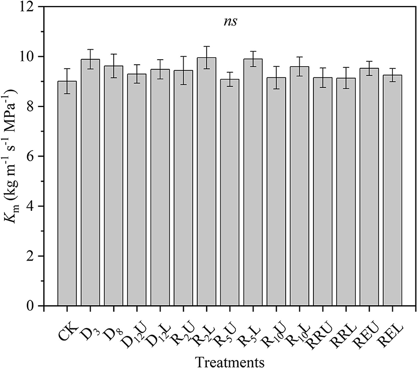
Figure 1. Maximum stem-specific hydraulic conductivity (Km) for all treatments. CK, control group; D3, mild drought group; D8, moderate drought group; D12U, upper part of the severe drought group; D12L, lower part of the severe drought group; R2U, upper part of the 2-day-rewatering group; R2L, lower part of the 2-day-rewatering group; R5U, upper part of the 5-day-rewatering group; R5L, lower part of the 5-day-rewatering group; R10U, upper part of the 10-day-rewatering group; R10L, lower part of the 10-day-rewatering group; RRU, upper part of the group, in which rewatering occurred until rebudding was present; RRL, lower part of the group, in which rewatering occurred until rebudding was present; REU, upper part of the rewatering group to the end of the experiment; REL, lower part of the rewatering group to the end of the experiment. The data is represented by the mean ± 1 SE and n = 10. One-way ANOVA and Duncan multiple comparisons were performed to detect the differences among all the treatments; ns indicates no significant difference.
The Weibull CDF accurately fit the HVC according to the coefficients of determination (R2 = 0.999, P < 0.01). The result of the fitting is as follows:
D12U and R2U to REU were along the right side of Ψl (no return zone), while the other treatments were along the left side of Ψl (recoverable zone). The LC of CK, RRL, and REL were similar to LCe, while D8 was close to Ψm, and D12L and D12U were on both sides of Ψl (Figure 2).
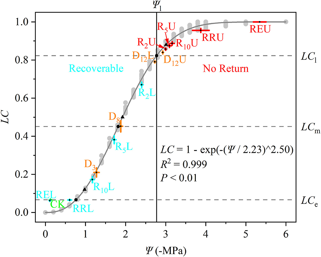
Figure 2. Hydraulic vulnerability curve (gray solid line) for Robinia pseudoacacia, which is fitted from 10 saplings belonging to CK (light gray points). The stem water potential (Ψ, –MPa) and loss of conductivity (LC) for all of the treatments are marked in the figure. The data is represented by the mean ± 1 SE and n = 10. CK, control group; D3, mild drought group; D8, moderate drought group; D12U, upper part of the severe drought group; D12L, lower part of the severe drought group; R2U, upper part of the 2-day-rewatering group; R2L, lower part of the 2-day-rewatering group; R5U, upper part of the 5-day-rewatering group; R5L, lower part of the 5-day-rewatering group; R10U, upper part of the 10-day-rewatering group; R10L, lower part of the 10-day-rewatering group; RRU, upper part of the group in which rewatering occurred until rebudding was present; RRL, lower part of the group in which rewatering occurred until rebudding was present; REU, upper part of the group in which rewatering occurred until the end of the experiment; REL, lower part of the group in which rewatering occurred until the end of the experiment. Ψe, Ψm, and Ψl are bottom up in the black circles. In addition, LCe, LCm, and LCl (gray dash lines) are the corresponding LC of the Ψe, Ψm, and Ψl. Black triangles indicate Ψ12, Ψ50, and Ψ88. Ψ at Ψl (black vertical solid line) separates the curve into two parts; the left part is recoverable, while the right part cannot be recovered.
Based on Figure 2, the differences among the CK, RRL, REL, and Ψe, between D8 and Ψm, among D12L, D12U, and Ψl (Figure 3), were further examined. We tested that CK and REL do not have a noticeable difference; however, CK and REL have significant differences with RRL in Ψ. In addition, CK, RRL, and REL are significantly smaller in Ψ than Ψe. Meanwhile, for the LC of CK, RRL, and REL, there is a noticeable difference with LCe. Ψ and LC of D8 are equal to Ψm and LCm, respectively. Ψl and LCl are significantly larger than Ψ and LC of D12L, although they are significantly smaller than those of D12U, respectively.
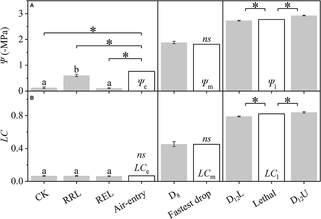
Figure 3. Differences among the CK, RRL, REL, and Ψe, between D8 and Ψm, and among D12L, Ψl, and D12U for the stem water potential (Ψ, A) and loss of conductivity (LC, B). CK, control group; D8, moderate drought group; D12U, upper part of the severe drought group; D12L, lower part of the severe drought group; RRL, lower part of the group in which rewatering occurred until rebudding was present; REL, lower part of the group in which rewatering occurred until the end of the experiment. The data that belongs to CK, RRL, REL, D8, D12L, and D12U are represented by the mean ± 1 SE and n = 10. Data of the three key points are signified by the calculated results via the DM. One-way ANOVA and Duncan multiple comparisons were performed to detect the differences among CK, RRL, and REL; different letters indicate significant differences where P < 0.05. The one-sample t-test was used to detect the difference between the calculated and experimental results; ns indicates no significant difference; the symbol *P < 0.05.
Subsequently, we tested the differences among the treatments (Figure 4). To make the results more intuitive and scientific, we separated the treatments into three groups. Figures 4A,B depict that Ψ and LC significantly increased for CK, D3, and D8 by increasing the drought stress. Figures 4C,D demonstrate that for D12U and R2U to REU, by increasing the rewatering time, there is no apparent change for Ψ and LC (D12U to R10U); then, Ψ and LC increased to a high level (R10U to REU). However, by further increasing the rewatering time, Ψ and LC of D12L and R2L to REL decreased significantly (Figures 4E,F).
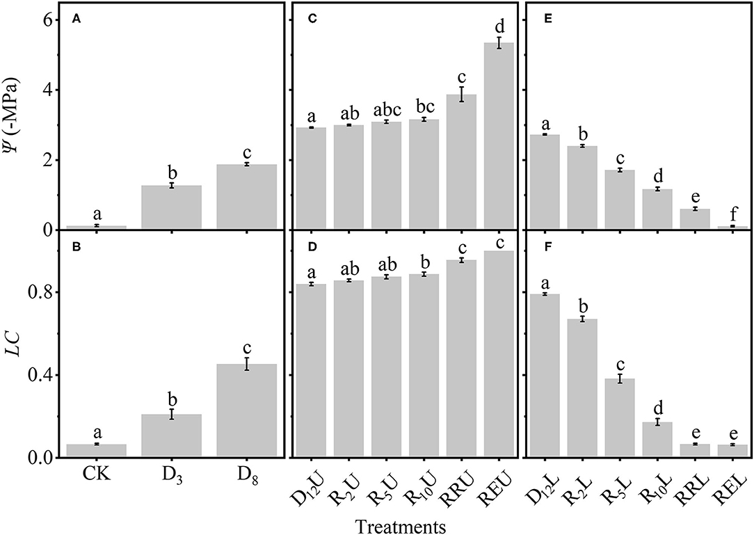
Figure 4. Differences among: CK, D3, D8 (A); D12U, R2U to REU (C); D12L, R2L to REL (E) for the stem water potential (Ψ). The loss of conductivity (LC) differences among CK, D3, D8 (B); D12U, R2U to REU (D); and D12L, R2L to REL (F). CK, control group; D3, mild drought group; D8, moderate drought group; D12U, upper part of the severe drought group; D12L, lower part of the severe drought group; R2U, upper part of the 2-day-rewatering group; R2L, lower part of the 2-day-rewatering group; R5U, upper part of the 5-day-rewatering group; R5L, lower part of the 5-day-rewatering group; R10U, upper part of the 10-day-rewatering group; R10L, lower part of the 10-day-rewatering group; RRU, upper part of the group, in which rewatering occurred until rebudding was present; RRL, lower part of the group, in which rewatering occurred until rebudding was present; REU, upper part of the group, in which rewatering occurred until the end of the experiment; REL, lower part of the group, in which rewatering occurred until the end of the experiment. The data is represented by the mean ± 1 SE, and n = 10. One-way ANOVA and Tamhane multiple comparisons were performed to detect the differences. In addition, different letters indicate significant differences, where P < 0.05.
With the increase in the drought stress (Ψs), Ψ increased linearly (R2 = 0.9999, P < 0.001; Figure 5A), Ks and E decreased linearly (R2 = 0.8898, P < 0.05; Figure 5B). WG and WL decreased significantly, while the difference between WG and WL reached the minimum value at D8 (Figure 6).
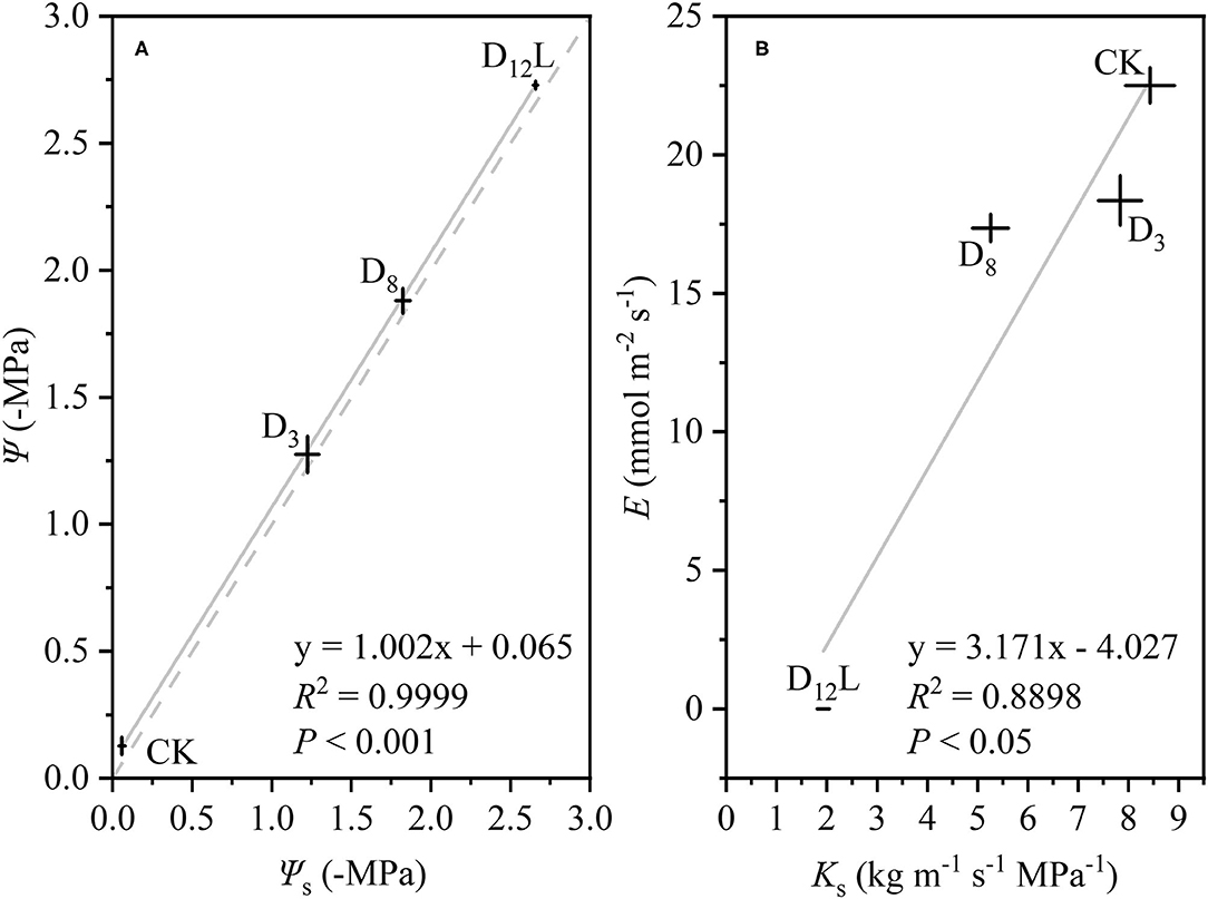
Figure 5. The relationship between soil water potential (Ψs, –MPa) and stem water potential (Ψ, –MPa), (A) between stem-specific hydraulic conductivity (Ks, kg m−1 s−1 MPa−1) and transpiration rate (E, mol m−2 s−1), (B) in CK, D3, D8, and D12L. CK, control group; D3, mild drought group; D8, moderate drought group; D12L, lower part of the severe drought group. The data is represented by the mean ± 1 SE and n = 10. Light gray line stands for the linear regression of the points, and light gray dash line stands for Ψ = Ψs.

Figure 6. Water gain (WG) and water loss (WL) of CK, D3, D8, and D12. CK, control group; D3, mild drought group; D8, moderate drought group; D12L, lower part of the severe drought group. Black circles represent WG, gray triangles indicate WL, and light gray squares represent the difference between WG and WL. The data is represented by the mean ± 1 SE and n = 10. One-way ANOVA and Duncan multiple comparisons were performed to detect the differences among WG and WL and WG – WL in CK, D3, D8, and D12L. In addition, different letters indicate significant differences, where P < 0.05.
Using the key points calculated using the DM, we divided the HVC into four parts (Figure 7). In parts (1) and (4), when the water potential becomes larger, the change of hydraulic conductivity is less than that in parts (2) and (3). In other words, a slight change in (1) and (4) is observed, while a straight drop is observed in (2) and (3).
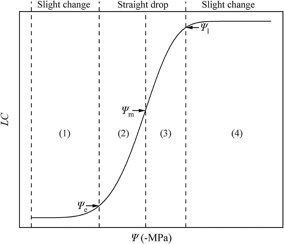
Figure 7. Hydraulic vulnerability curve diagram. The water potential is represented by Ψ, and the loss of conductivity is represented by LC. There are four periods in the HVC: (1) stationary period, (2) accelerated decline period, (3) decelerated decline period, (4) and platform period. These are separated by three key points: air-entry point (Ψe), fastest drop point (Ψm), and upper inflection point (Ψl).
The visible periods included D8, D12, RR, and RE. The separatrix, new buds, and new leaves are clearly visible in Supplementary Figure 1.
Discussion
Drought Did Not Change the Water Transport Efficiency
There was no significant difference in the Km for all the treatments in this research (Figure 1). This indicates that during the experiment, the xylem structure of R. pseudoacacia did not have a noticeable change (Choat et al., 2012), and the differences of the xylem function were completely caused by the treatments. However, our treatments did not change the water transport efficiency (Figure 1), according to the xylem efficiency-safety tradeoff, which meant that a balance existed between hydraulic efficiency and safety (Gleason et al., 2016; Liu et al., 2019). It can be concluded that the water transport safety of R. pseudoacacia has not changed significantly during the experiment; thus, we can only use one HVC to examine the hydraulic vulnerability for all the treatments. Notably, some researches indicated that the “air-injection” method may be prone to artifacts if the maximum length of the xylem vessels is not considered when preparing the samples for conducting the measurements (Ennajeh et al., 2011). However, this research was based on 4-month-old saplings, it is impossible to have a long conduit like a tree, according to the shape of our HVC (Figure 2) and previous researches (Zhu et al., 2018; Li et al., 2019, 2020; Liu et al., 2020), we convince that the 30-cm-long segments had no open vessels, so that the “air-injection” method did not cause experimental artifacts in this research. Moreover, the “air-injection” method can accurately control the stem water potential, and it can improve the precision of the HVC (Sergent et al., 2020).
Calculated Result From Differential Method Can Better Estimate the Experimental Results
With the rise in the drought stress, Ψ and LC of R. pseudoacacia increased (Figures 2, 4A,B). After rewatering, Ψ and LC of the stem above the separatrix did not recover. However, Ψ and LC were maintained at the initial level from D12U to R10U, after which Ψ and LC increased significantly, and then achieved full embolism (Figures 4C,D). In addition, the stem below the separatrix began to recover (Figures 4E,F). According to the hydraulic segmentation hypothesis, plants maintained the hydraulic status of the stems by reducing the transpiration through defoliation; thus, Ψ and LC of xylem exhibited no apparent change. The question arises to why D12L can recover from the drought stress after rewatering whereas D12U cannot. It is possible that the water resource of D12U can get through the hydraulic conductance. However, this would never meet their metabolic needs, let alone rebudding, even if they were rewatered, in which they “passed the point of no return.” In contrast, the water resource of D12L that was gained from the hydraulic conductance achieved their metabolic needs (the value was ~54.89 × 10⁻⁶ kg s−1, Figure 6). After recovery, they can rebud. By comparing these two parts (Figure 2), we determined that, although their Ψ and LC are close, their responses after rewatering were inconsistent. Like the “squeeze theorem” (Wang and Jiang, 2014), the lethal point of R. pseudoacacia was at a point that ranged from 2.73 to 2.93 MPa, and the corresponding LC ranged from 0.79 to 0.84 (Figure 3). Meanwhile, Ψl (=2.77 MPa) that was obtained by the DM was between 2.73 and 2.93, and LCl (=0.82) ranged from 0.79 to 0.84. Therefore, we demonstrated that Ψ of D12L < Ψl < Ψ of D12U (P < 0.05) and LC of D12L < LCl < LC of D12U (P < 0.05). In addition, Ψ88 overestimated the lethal point (Figure 3). Based on our experimental result, by combining the definition and geometric meanings of the lethal point, we recommend that Ψl, which is obtained by the DM, is the lethal point (the point of no return) of R. pseudoacacia.
We tested that the LC of CK, RRL, and REL were concentrated next to LCe (Figure 3B); however, their Ψ values were significantly smaller than Ψe. This indicated that when LC was reduced to the control level, although Ψ continued to decrease, the LC would never be reduced but maintained at a certain level. In other words, the Ks for CK and REL were still lower than Km. This may be because R. pseudoacacia has some natural embolism that was not induced by stress (Li et al., 2020). Consequently, the actual Km is smaller than the theoretical Km. Natural embolism may exist because R. pseudoacacia is anisohydric, and its Ψ and LC changes with the changing environment (Li et al., 2019). Moreover, recovery of natural embolism would consume a significant amount of resources; however, it would produce less benefits, which goes against the resource trade-off theory. Conversely, when facing drought stress, at the period when Ψ is raised from 0 to Ψe, because of natural embolism, the Ks would never decline significantly. Nevertheless, when Ψ > Ψe, Ks starts to decrease. This conforms with our definition of the air-entry point. Therefore, Ψe is possibly the ultimate Ψ that can enable the plant to maintain the actual Km. Consequently, we recommend to have Ψe as the air-entry point of R. pseudoacacia, which is obtained by the DM.
In addition, we observed that Ψ and Ψm as well as LC and LCm have no noticeable difference at D8 (Figure 3). It was hypothesized that under the increasing drought stress (Figure 5A), Ks and E decreased linearly (Figure 5B), WG and WL decreased. However, the difference between WG and WL reached the minimum value at D8 (Figure 6). At that point, the net water resource xylem was gained from the soil (~8.83 × 10⁻⁶ kg s−1, Figure 6), and its metabolic requirements cannot be satisfied (~54.89 × 10⁻⁶ kg s−1, Figure 6). The plant can only meet the water demand by reducing the water content of xylem, leading to rapid diffusion of embolism, and at that point, LC increases the fastest. Therefore, during D8-D12, the leaves started to dry and fall off. In addition, they form a hydraulic segmentation, which ensures metabolic water at the expense of transpiration, thereby slowing down the increase of the LC. Accordingly, we can determine that Ψm is the fastest drop point of R. pseudoacacia.
Furthermore, we tested and compared the results obtained by Hammond et al. (2019) with those of the DM, and the results were found to be the same. Therefore, we can conclude that the differences between the experimental and calculated results can be attributed to the linear progressive method of the “turning melody into straightness,” and the DM can eliminate the differences. A significant amount of work is required to perfect this method. As indicated by Hammond et al. (2019), continued experimentation is necessary to assess the different tree species, populations, and individuals in different ontogeny stages.
Four Periods of HVC for Better Understanding of Hydraulic State
By applying Ψe, Ψm, and Ψl, we can divide the HVC into four periods (Figure 7), including (1) the stationary period (0 ≤ Ψ < Ψe). Currently, the Ψ is low, and the Ks may be at the theoretical Km, similar to P. taeda (Hammond et al., 2019), or at the actual Km, similar to R. pseudoacacia. When the plants are facing drought stress, the absolute value of Ψ increases, whereas Ks slightly decreases or remains largely unchanged. As Ψ increases to more than Ψe, the plants can no longer maintain the Ks at the theoretical or actual Km. (2) From this point forward, the entry of air causes the hydraulic conductivity to decrease linearly. In addition, the stem of the plant enters a period of accelerated decline from the stationary period (Ψe ≤ Ψ < Ψm), during which the aggravation of stress continues to cause Ψ to increase. In other words, a slight change in Ψ will cause a large drop in the hydraulic conductivity. This is due to the increasing drought stress and the undiminished transpiration of the entire plant. In particular, when Ψ = Ψm, the hydraulic conductivity exhibits the fastest drop rate, after which it proceeds to a period of (3) decelerated decline (Ψm ≤ Ψ < Ψl). In this period, as mentioned in the hydraulic segmentation hypothesis, the water resource that xylem gained from the soil cannot satisfy the transpiration and metabolic needs; hence, the leaves begin to dry and fall off. To satisfy the stem metabolism and protect the stem from severe embolism, the increase of Ψ and LC slows down (before the lethal point). (4) When Ψl ≤ Ψ, although the branches of the plant do not completely lose their hydraulic conductivity, they lose their ability to recover. At this stage, the stem of the plant enters the platform period until Ψ arrives at the highest point. These four periods belong to the same vulnerability curve due to their different ecological significance and mathematical properties. Our results prove again the significance of the HVC in studying plant responses to drought. Therefore, we strongly recommend that research related to the HVC should be focused for a certain period, and further investigations must be performed on the mechanisms.
Ball (2016) placed an emphasis on the models and parameters from the fitting curves and implied that the models or calculated parameters from the models need to be more practical. From the drought-rewatering experiment, we determined the lethal point, air entry point, and fastest drop point of R. pseudoacacia. We also verified that the three points can be represented by Ψl, Ψe, and Ψm, which can be calculated from the DM, respectively. According to the Ψ values, we divided the HVC into four periods: (1) 0 ≤ Ψ < Ψe, (2) Ψe ≤ Ψ < Ψm, (3) Ψm ≤ Ψ < Ψl, and (4) Ψl ≤ Ψ. More experimental and theoretical studies to address the HVC are urgently needed in the future to better understand the hydraulic state of the plants.
Data Availability Statement
The original contributions presented in the study are included in the article/Supplementary Materials, further inquiries can be directed to the corresponding authors.
Author Contributions
XL designed the research, conducted the field and laboratory measurements, and analyzed the data. ND and HW designed the research and secured funding. NW, RC, and HS contributed to the laboratory measurements and the data analysis. FW and XS conducted the data analysis. RW provided ideas for writing. XL wrote the manuscript that was intensively edited by all of the authors.
Funding
This research was funded by the Basic Work of the Ministry of Science and Technology, China (No. 2015FY210200-11), the National Natural Science Foundation of China (Nos. 31400173 and 31600313), and the Research Foundation of the Qingdao Forest Ecosystem (No. 11200005071603).
Conflict of Interest
The authors declare that the research was conducted in the absence of any commercial or financial relationships that could be construed as a potential conflict of interest.
Acknowledgments
We wish to thank Editage (www.editage.com) for English language editing.
Supplementary Material
The Supplementary Material for this article can be found online at: https://www.frontiersin.org/articles/10.3389/fpls.2021.627403/full#supplementary-material
Supplementary Figure 1. The visible treatments, which include: D8, the moderate drought group; D12, the severe drought group; RR, the group in which rewatering occurred until rebudding was present; and RE, the group in which rewatering occurred until the end of the experiment. The separatrix, new buds, and new leaves are marked.
References
Adams, H. D., Guardiola-Claramonte, M., Barron-Gafford, G. A., Villegas, J. C., Breshears, D. D., Zou, C. B., et al. (2009). Temperature sensitivity of drought-induced tree mortality portends increased regional die-off under global-change-type drought. Proc. Natl. Acad. Sci. U.S.A. 106, 7063–7066. doi: 10.1073/pnas.0901438106
Adams, H. D., Zeppel, M. J. B., Anderegg, W. R. L., Hartmann, H., Landhäusser, S. M., Tissue, D. T., et al. (2017). A multi-species synthesis of physiological mechanisms in drought-induced tree mortality. Nat. Ecol. Evol. 1, 1285–1291. doi: 10.1038/s41559-017-0248-x
Adnadević B. K Baroš Z. Z. (2013). Application of Weibull distribution function for modelling the isothermal kinetics of the titanium-oxo-alkoxy clusters growth. Thermochim Acta 551, 46–52. doi: 10.1016/j.tca.2012.10.011
Anderegg, W. R. L., Berry, J. A., Smith, D. D., Sperry, J. S., Anderegg, L. D. L., and Field, C. B. (2012). The roles of hydraulic and carbon stress in a widespread climate-induced forest die-off. Proc. Natl. Acad. Sci. U.S.A. 109, 233–237. doi: 10.1073/pnas.1107891109
Anderegg, W. R. L., and Meinzer, F. C. (2015). “Wood anatomy and plant hydraulics in a changing climate,” in Functional and Ecological Xylem Anatomy, ed U. Hacke (Cham: Springer), 235–253.
Ball, P. (2016). The mathematics of science's broken reward system. Nature. doi: 10.1038/nature.2016.20987
Benito Garzón, M., González Muñoz, N., Wigneron, J. P., Moisy, C., Fernández-Manjarrés, J., and Delzon, S. (2018). The legacy of water deficit on populations having experienced negative hydraulic safety margin. Glob. Ecol. Biogeogr. 27, 346–356. doi: 10.1111/geb.12701
Brodribb, T. J., and Cochard, H. (2009). Hydraulic failure defines the recovery and point of death in water-stressed conifers. Plant Physiol. 149, 575–584. doi: 10.1104/pp.108.129783
Choat, B., Jansen, S., Brodribb, T. J., Cochard, H., Delzon, S., Bhaskar, R., et al. (2012). Global convergence in the vulnerability of forests to drought. Nature 491:752. doi: 10.1038/nature11688
Corcuera, L., Cochard, H., Gil-Pelegrin, E., and Notivol, E. (2011). Phenotypic plasticity in mesic populations of Pinus pinaster improves resistance to xylem embolism (P50) under severe drought. Trees 25, 1033–1042. doi: 10.1007/s00468-011-0578-2
Delzon, S., and Cochard, H. (2014). Recent advances in tree hydraulics highlight the ecological significance of the hydraulic safety margin. New Phytol. 203, 355–358. doi: 10.1111/nph.12798
Dietrich, L., Delzon, S., Hoch, G., and Kahmen, A. (2019). No role for xylem embolism or carbohydrate shortage in temperate trees during the severe 2015 drought. J. Ecol. 107, 334–349. doi: 10.1111/1365-2745.13051
Domec, J. C., and Gartner, B. L. (2001). Cavitation and water storage capacity in bole xylem segments of mature and young Douglas-fir trees. Trees 15, 204–214. doi: 10.1007/s004680100095
Dulamsuren, C., Abilova, S. B., Bektayeva, M., Eldarov, M., Schuldt, B., Leuschner, C., et al. (2018). Hydraulic architecture and vulnerability to drought-induced embolism in southern boreal tree species of Inner Asia. Tree Physiol. 39, 463–473. doi: 10.1093/treephys/tpy116
Easterling, D. R., Meehl, G. A., Parmesan, C., Changnon, S. A., Karl, T. R., and Mearns, L. O. (2000). Climate extremes: observations, modeling, and impacts. Science 289, 2068–2074. doi: 10.1126/science.289.5487.2068
Ennajeh, M., Nouiri, M., Khemira, H., and Cochard, H. (2011). Improvement to the air-injection technique to estimate xylem vulnerability to cavitation. Trees 25, 705–710. doi: 10.1007/s00468-011-0548-8
Fuenzalida, T. I., Bryant, C. J., Ovington, L. I., Yoon, H. J., Oliveira, R. S., Sack, L., et al. (2019). Shoot surface water uptake enables leaf hydraulic recovery in Avicennia marina. New Phytol. 224, 1504–1511. doi: 10.1111/nph.16126
Ge, C., Yu, X., Kan, M., and Qu, C. (2017). Adaption of Ulva pertusa to multiple-contamination of heavy metals and nutrients: biological mechanism of outbreak of Ulva sp. green tide. Marine Pollut. Bull. 125, 250–253. doi: 10.1016/j.marpolbul.2017.08.025
Gimbel, K. F., Felsmann, K., Baudis, M., Puhlmann, H., Gessler, A., Bruelheide, H., et al. (2015). Drought in forest understory ecosystems – a novel rainfall reduction experiment. Biogeosciences 12, 961–975. doi: 10.5194/bg-12-961-2015
Gleason, S. M., Westoby, M., Jansen, S., Choat, B., Hacke, U. G., Pratt, R. B., et al. (2016). Weak tradeoff between xylem safety and xylem-specific hydraulic efficiency across the world's woody plant species. New Phytol. 209, 123–136. doi: 10.1111/nph.13646
Hammond, W. M., Yu, K., Wilson, L. A., Will, R. E., Anderegg, W. R. L., and Adams, H. D. (2019). Dead or dying? Quantifying the point of no return from hydraulic failure in drought-induced tree mortality. New Phytol. 223, 1834–1843. doi: 10.1111/nph.15922
Hartmann, H., Moura, C. F., Anderegg, W. R., Ruehr, N. K., Salmon, Y., Allen, C. D., et al. (2018). Research frontiers for improving our understanding of drought-induced tree and forest mortality. New Phytol. 218, 15–28. doi: 10.1111/nph.15048
Högy, P., Poll, C., Marhan, S., Kandeler, E., and Fangmeier, A. J. F. C. (2013). Impacts of temperature increase and change in precipitation pattern on crop yield and yield quality of barley. Food Chem. 136, 1470–1477. doi: 10.1016/j.foodchem.2012.09.056
Kannenberg, S. A., Novick, K. A., and Phillips, R. P. (2019). Anisohydric behavior linked to persistent hydraulic damage and delayed drought recovery across seven North American tree species. New Phytol. 222, 1862–1872. doi: 10.1111/nph.15699
Li, Q., Wang, N., Liu, X., Liu, S., Wang, H., Zhang, W., et al. (2019). Growth and physiological responses to successional water deficit and recovery in four warm-temperate woody species. Physiol. Plantarum 167:645–660. doi: 10.1111/ppl.12922
Li, Q., Zhao, M., Wang, N., Liu, S., Wang, J., Zhang, W., et al. (2020). Water use strategies and drought intensity define the relative contributions of hydraulic failure and carbohydrate depletion during seedling mortality. Plant Physiol. Biochem. 153, 106–118. doi: 10.1016/j.plaphy.2020.05.023
Liu, H., Gleason, S. M., Hao, G., Hua, L., He, P., Goldstein, G., et al. (2019). Hydraulic traits are coordinated with maximum plant height at the global scale. Sci. Adv. 5:eaav1332. doi: 10.1126/sciadv.aav1332
Liu, X., Li, Q., Wang, F., Sun, X., Wang, N., Song, H., et al. (2020). Weak tradeoff and strong segmentation among plant hydraulic traits during seasonal variation in four woody species. Front. Plant Sci. 11:585674. doi: 10.3389/fpls.2020.585674
Liu, Y., Wang, A., An, Y., Lian, P., Wu, D., Zhu, J., et al. (2018). Hydraulics play an important role in causing low growth rate and dieback of aging Pinus sylvestris var. mongolica trees in plantations of Northeast China. Plant Cell Environ. 41, 1500–1511. doi: 10.1111/pce.13160
Martinez-Vilalta, J., and Pinol, J. (2002). Drought-induced mortality and hydraulic architecture in pine populations of the NE Iberian Peninsula. Forest Ecol. Manage. 161, 247–256. doi: 10.1016/S0378-1127(01)00495-9
Martin-StPaul, N., Delzon, S., and Cochard, H. (2017). Plant resistance to drought depends on timely stomatal closure. Ecol. Lett. 20, 1437–1447. doi: 10.1111/ele.12851
Meinzer, F. C., Johnson, D. M., Lachenbruch, B., McCulloh, K. A., and Woodruff, D. R. (2009). Xylem hydraulic safety margins in woody plants: coordination of stomatal control of xylem tension with hydraulic capacitance. Funct. Ecol. 23, 922–930. doi: 10.1111/j.1365-2435.2009.01577.x
Nardini, A., Battistuzzo, M., and Savi, T. (2013). Shoot desiccation and hydraulic failure in temperate woody angiosperms during an extreme summer drought. New Phytol. 200, 322–329. doi: 10.1111/nph.12288
O'Grady, A. P., Mitchell, P. J. M., Pinkard, E. A., and Tissue, D. T. (2013). Thirsty roots and hungry leaves: unravelling the roles of carbon and water dynamics in tree mortality. New Phytol. 200, 294–297. doi: 10.1111/nph.12451
Oliveira, R. S., Costa, F. R. C., van Baalen, E., de Jonge, A., Bittencourt, P. R., Almanza, Y., Barros, F. D. V., et al. (2019). Embolism resistance drives the distribution of Amazonian rainforest tree species along hydro-topographic gradients. New Phytol. 221, 1457–1465. doi: 10.1111/nph.15463
Pammenter, N. W., and van der Willigen, C. (1998). A mathematical and statistical analysis of the curves illustrating vulnerability of xylem to cavitation. Tree Physiol. 18, 589–593. doi: 10.1093/treephys/18.8-9.589
Santiago, L. S., de Guzman, M. E., Baraloto, C., Vogenberg, J. E., Brodie, M., Hérault, B., et al. (2018). Coordination and trade-offs among hydraulic safety, efficiency and drought avoidance traits in Amazonian rainforest canopy tree species. New Phytol. 218, 1015–1024. doi: 10.1111/nph.15058
Scholz, F. G., Bucci, S. J., and Goldstein, G. (2014). Strong hydraulic segmentation and leaf senescence due to dehydration may trigger die-back in Nothofagus dombeyi under severe droughts: a comparison with the co-occurring Austrocedrus chilensis. Trees. 28, 1475–1487. doi: 10.1007/s00468-014-1050-x
Schreel, J. D. M., and Steppe, K. (2019). Foliar water uptake changes the world of tree hydraulics. NPJ Climate Atmo. Sci. 2:1. doi: 10.1038/s41612-018-0060-6
Sergent, A. S., Varela, S., Barigah, T., Badel, E., Cochard, H., Dalla-Salda, G., et al. (2020). A comparison of five methods to assess embolism resistance in trees. Forest Ecol. Managem. 468, 118–175. doi: 10.1016/j.foreco.2020.118175
Sevanto, S., Mcdowell, N. G., Dickman, L. T., Pangle, R., and Pockman, W. T. (2014). How do trees die? A test of the hydraulic failure and carbon starvation hypotheses. Plant Cell Environ. 37, 153–161. doi: 10.1111/pce.12141
Sparks, J. P., and Black, R. A. (1999). Regulation of water loss in populations of Populus trichocarpa: the role of stomatal control in preventing xylem cavitation. Tree Physiol. 19, 453–459. doi: 10.1093/treephys/19.7.453
Sperry, J. S., Tyree, M. T., and Donnelly, J. R. (1988). Vulnerability of xylem to embolism in a mangrove vs an inland species of Rhizophoraceae. Physiol. Plantarum 74, 276–283. doi: 10.1111/j.1399-3054.1988.tb00632.x
Torres-Ruiz, J. M., Cochard, H., Choat, B., Jansen, S., López, R., Tomáškov,á, I., et al. (2017). Xylem resistance to embolism: presenting a simple diagnostic test for the open vessel artefact. New Phytol. 215, 489–499. doi: 10.1111/nph.14589
Tyree, M. T., and Sperry, J. S. (1988). Do woody plants operate near the point of catastrophic xylem dysfunction caused by dynamic water stress? Plant Physiol. 88, 574–580. doi: 10.1104/pp.88.3.574
Wang, N., Zhao, M., Li, Q., Liu, X., Song, H., Peng, X., et al. (2020). Effects of defoliation modalities on plant growth, leaf traits, and carbohydrate allocation in Amorpha fruticosa L. and Robinia pseudoacacia L. seedlings. Ann. Forest Sci. 77:53. doi: 10.1007/s13595-020-00953-1
Wason, J. W., Anstreicher, K. S., Stephansky, N., Huggett, B. A., and Brodersen, C. R. (2018). Hydraulic safety margins and air-seeding thresholds in roots, trunks, branches and petioles of four northern hardwood trees. New Phytol. 219, 77–88. doi: 10.1111/nph.15135
Yin, X., Sterck, F., and Hao, G. (2018). Divergent hydraulic strategies to cope with freezing in co-occurring temperate tree species with special reference to root and stem pressure generation. New Phytol. 219, 530–541. doi: 10.1111/nph.15170
Zhang, Y., Rockwell, F. E., Graham, A. C., Alexander, T., and Holbrook, N. M. (2016). Reversible leaf xylem collapse: a potential “circuit breaker” against cavitation. Plant Physiol. 172, 2261–2274. doi: 10.1104/pp.16.01191
Zhu, S., He, P., Li, R., Fu, S., Lin, Y., Zhou, L., et al. (2018). Drought tolerance traits predict survival ratio of native tree species planted in a subtropical degraded hilly area in South China. Forest Ecol. Manage. 418, 41–46. doi: 10.1016/j.foreco.2017.09.016
Glossary
A, average cross-sectional area for both ends of the stem; CDF, cumulative distribution function; CK, control group; D3, mild drought group; D8, moderate drought group; D12, severe drought group; D12L, the lower part of the sapling in the severe drought group; D12U, the upper part of the sapling in the severe drought group; DM, differential method; E, transpiration rate, HVC, hydraulic vulnerability curve; Km, maximum stem-specific hydraulic conductivity; Ks, stem-specific hydraulic conductivity; L, length of the segment; LC, loss of conductivity; LCe, loss of conductivity at air-entry point; LCl, loss of conductivity at upper inflection point; LCm, loss of conductivity at fastest drop point; LED, light emitting diode; m, mass of water through the segment; p, intensity of the water pressure across the segment; PPFD, photosynthetic photo flux density; Qm, mass of water per unit of time through a segment; R2, the group of 2 days after rewatering; R2L, the lower part of the sapling in the group of 2 days after rewatering; R2U, the upper part of the sapling in the group of 2 days after rewatering; R5, the group of 5 days after rewatering; R5L, the lower part of the sapling in the group of 5 days after rewatering; R5U, the upper part of the sapling in the group of 5 days after rewatering; R10, the group of 10 days after rewatering; R5L, the lower part of the sapling in the group of 10 days after rewatering; R5U, the upper part of the sapling in the group of 10 days after rewatering; RE, the group of rewatering occurred until the end of the experiment; REL, the lower part of the sapling in the group of rewatering occurred until the end of the experiment; REU, the upper part of the sapling in the group of rewatering occurred until the end of the experiment; RR, the group of rewatering occurred until rebudding was present; RRL, the lower part of the sapling in the group of rewatering occurred until rebudding was present; RRU, the upper part of the sapling in the group of rewatering occurred until rebudding was present; T, time of the water conductance at maximum stem-specific hydraulic conductivity; t, time for the conductance measurement; TM, traditional method; WG, water gain; WL, water loss; Ψ, stem water potential; Ψs, soil water potential; Ψe, air-entry point; Ψl, upper inflection point; Ψm, fastest drop point; Ψ12, the pressure with a 12% hydraulic conductivity loss; Ψ50, the pressure with a 50% hydraulic conductivity loss; Ψ88, the pressure with a 88% hydraulic conductivity loss; ΔΨ, the difference between soil water potential and stem water potential.
Keywords: calculated result, differential method, experimental result, hydraulic, loss of conductivity, water potential
Citation: Liu X, Wang N, Cui R, Song H, Wang F, Sun X, Du N, Wang H and Wang R (2021) Quantifying Key Points of Hydraulic Vulnerability Curves From Drought-Rewatering Experiment Using Differential Method. Front. Plant Sci. 12:627403. doi: 10.3389/fpls.2021.627403
Received: 11 November 2020; Accepted: 08 January 2021;
Published: 02 February 2021.
Edited by:
Lars Hendrik Wegner, Foshan University, ChinaReviewed by:
Thorsten M. Knipfer, University of British Columbia, CanadaQing Ye, Chinese Academy of Sciences, China
Copyright © 2021 Liu, Wang, Cui, Song, Wang, Sun, Du, Wang and Wang. This is an open-access article distributed under the terms of the Creative Commons Attribution License (CC BY). The use, distribution or reproduction in other forums is permitted, provided the original author(s) and the copyright owner(s) are credited and that the original publication in this journal is cited, in accordance with accepted academic practice. No use, distribution or reproduction is permitted which does not comply with these terms.
*Correspondence: Ning Du, ZHVuaW5nX3NkdUAxMjYuY29t; Hui Wang, d2FuZ2h1aTEyMjdAc2R1LmVkdS5jbg==