 Hui Feng1,2
 Lizhong Xiong
 Wanneng Yang
- 1National Key Laboratory of Crop Genetic Improvement, National Center of Plant Gene Research, Agricultural Bioinformatics Key Laboratory of Hubei Province, and College of Engineering, Huazhong Agricultural University, Wuhan, China
- 2Britton Chance Center for Biomedical Photonics, Wuhan National Laboratory for Optoelectronics, and Key Laboratory of Ministry of Education for Biomedical Photonics, Department of Biomedical Engineering, Huazhong University of Science and Technology, Wuhan, China
Pigments absorb light, transform it into energy, and provide reaction sites for photosynthesis; thus, the quantification of pigment distribution is vital to plant research. Traditional methods for the quantification of pigments are time-consuming and not suitable for the high-throughput digitization of rice pigment distribution. In this study, using a hyperspectral imaging system, we developed an integrated image analysis pipeline for automatically processing enormous amounts of hyperspectral data. We also built models for accurately quantifying 4 pigments (chlorophyll a, chlorophyll b, total chlorophyll and carotenoid) from rice leaves and determined the important bands (700-760 nm) associated with these pigments. At the tillering stage, the R2 values and mean absolute percentage errors of the models were 0.827–0.928 and 6.94–12.84%, respectively. The hyperspectral data and these models can be combined for digitizing the distribution of the chlorophyll with high resolution (0.11 mm/pixel). In summary, the integrated hyperspectral image analysis pipeline and selected models can be used to quantify the chlorophyll distribution in rice leaves. The use of this technique will benefit rice functional genomics and rice breeding.
Introduction
Rice is a staple food for a majority of the world population (Zhang, 2007). To meet the increasing demand due to natural disasters, human factors and the increasing world population on rice growth and yield, it is important to breed new rice varieties. In breeding research, the plant phenotype is essential for the evaluation of breeding results and gene functional analysis (Yang et al., 2013; Jasinski et al., 2016; Montagnoli et al., 2016; Negi et al., 2016). Plants contain pigments such as chlorophylls and carotenoids, which absorb light and provide energy for photosynthesis (Blackburn, 1998b). Chlorophyll is the major nitrogenous substance in higher plants and can be used for measuring plant growth (Kochubey and Kazantsev, 2007; Xue and Yang, 2009). The amount of chlorophyll present also determines a plant's photosynthetic capability, productivity and yield potential (Carter, 1998; Xue and Yang, 2009). Thus, quantification of these pigments is vital for rice phenomics and rice research.
Traditional methods for the quantification of plant pigments, including spectrophotometry (Ergun et al., 2004), paper chromatography (Sporer et al., 1954), thin-layer chromatography (Sievers and Hynninen, 1977), and high-performance liquid chromatography (Yuan et al., 1997), are time-consuming, destructive and not suitable for high-throughput phenotyping. Plant pigments have different absorption peaks under different wavelengths, which means that their spectral reflectance characteristics can be used for evaluating or distinguishing pigments (Benedict and Swidler, 1961; Gamon and Surfus, 1999). Using spectroscopy and a portable chlorophyll meter, several spectral indices have been identified, which can be used for predicting plant chlorophyll content non-destructively. Blackburn et al. reported that the amount of canopy chlorophyll a and b is related to the original reflectance at 676 and 810 nm (Blackburn, 1998a; Blackburn and Pitman, 1999). Because derivatization can reduce the noise caused by illumination, soil background, and atmosphere (Collins, 1978; Baret et al., 1992), derivative spectra have also been found to be more sensitive to the chlorophyll content and more effective than the original spectral index (Le Maire et al., 2004). Moreover, spectral indices calculated by the red edge can provide a more accurate estimation of pigment content (Miller et al., 1990; Zou et al., 2011). Researchers have also found that the ratio and normalized spectral indices are closely related to the pigment content (Moss and Rock, 1991; Chappelle et al., 1992). Yi et al. used partial least square regression and found that the reflectance at 515–550 nm, 715 and 750 nm regions had high sensitivity for detecting the carotenoid contents of cotton (Yi et al., 2014). A recent study has used hyperspectral imagery to estimate the spatial variability in the chlorophyll and nitrogen content of rice, with an R2 of 0.69–0.82 (Moharana and Dutta, 2016). Researchers also used canopy reflectance to estimate the durum wheat nitrogen status, with an RMSECV of 19.3–36.3% (Thorp et al., 2017). Portable chlorophyll meters, such as CCM-200 (Chlorophyll Content Meter) and SPAD-502 (Soil and Plant Analyzer Development), are widely used for measuring the chlorophyll content; however, manually operated portable chlorophyll meters are relatively subjective, and spectroscopy techniques cannot be used to digitize the chlorophyll distribution in rice leaves. Moreover, we summarized the recent studies on chlorophyll or nitrogen quantification that used spectral techniques (Supplementary Table 1). These studies showed that few efforts have been made to handle massive amounts of hyperspectral data and automatically digitalize the chlorophyll distribution in individual rice leaves with high-resolution.
In this study, we developed an integrated image analysis pipeline that can process extremely large amounts of hyperspectral data and built models to accurately measure 4 rice leaf pigments: chlorophyll a, chlorophyll b, total chlorophyll, and carotenoid. Moreover, by combining the hyperspectral data and the selected models, the distribution of these 4 pigments can be digitized with high resolution.
Materials and Methods
Materials and Experimental Design
At the tillering stage, 10 rice accessions (BLUE STICK, Chenwan3hao, PSBRC82, Manawthukha, Guantuibaihe, Xianggu, Wumanggaonuo, La110, Diantun502, TB154E-TB-2, and Ajaya) were randomly selected from 533 rice core germplasm resources, and each accession was planted in 15 pots. The 15 pots were divided into 5 nitrogen application levels with 3 replicates: 0, 50, 100% (0.1 g nitrogen per kg soil), 150, and 200%. At the heading stage, 15 accessions (RP2151-173-1-8, MR77 (seberang), BASMATI 385, BLUE STICK, Chenwan3hao, PSBRC82, Manawthukha, Guantuibaihe, Xianggu, Wumanggaonuo, La110, Diantun502, TB154E-TB-2, Ajaya, and Bg90-2) were randomly selected from 533 rice core germplasm resources, and 10 replicates of each accession were planted under the same nitrogen level (0.1 g of nitrogen per kg of soil). To test the relationship between the leaf nitrogen and hyperspectral indices, 90 accessions (seen in Supplementary Table 2) were randomly selected from 533 rice core germplasm resources and measured by an auto discrete analyzer (Smartchen 200, France), SPAD-502, and hyperspectral imaging. Detailed genetic information about these SNPs can be downloaded from the “RiceVarMap” database (http://ricevarmap.ncpgr.cn/) (Narsai et al., 2013).
Hyperspectral Imaging System and Hyperspectral Indices Extraction
Three leaves were selected from the main stem of each rice plant and scanned using the hyperspectral imaging system, which consisted of 4 major parts (Figure 1A): a halogen lamp, a translation stage, a hyperspectral camera (HyperspecTM VNIR, Headwall Photonics, USA), and a computer (OXPCO3, Dell, USA). To scan three leaves of one main stem simultaneously, the field of view was set at 115 × 180 mm. The major configurations of the hyperspectral imaging system are shown in Figure 1B, and the main parameters of the hyperspectral imaging system are shown in Table 1. The data were continuously stored as a binary data stream to acquire and store the original hyperspectral data as rapidly as possible. For each sample, the data size was 1.15 GBit.
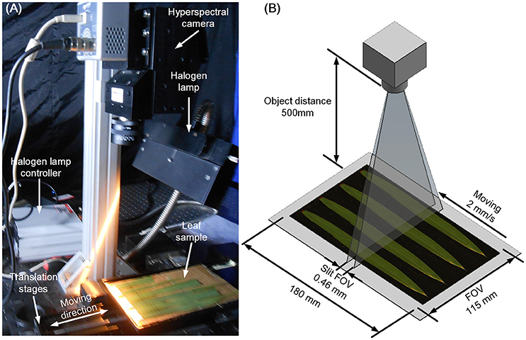
Figure 1. Hyperspectral imaging system (A) and schematic diagram (B).
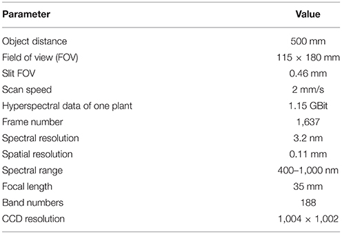
Table 1. Main parameters of the hyperspectral imaging system.
After data acquisition, the binary data stream was reorganized to build 188 hyperspectral images under different wavelengths (Figures 2A–C). To process the massive number of images automatically, an integrated hyperspectral image analysis pipeline was developed (Figure 3). The detailed image analysis pipeline designed by LabVIEW is shown in Supplementary Figures 1–11, which included the following steps: (1) Open one binary data stream with the band interleaved by line format: The size of the hyperspectral data cube was 188 × 1,004 (W) × 1,637 (H). (2) The binary data stream was reorganized to build 188 hyperspectral images. (3) Image processing and ROI extracting: After image division, gray conversion, image binarization, horizontal open operation, removal of large areas, removal of noise, region growing, and extraction of the area of interest, a region of interest (ROI) was extracted for each leaf (Figures 2E–N). (4) ROI reflectance extracting: 188 original average reflectance indices (R) were obtained. (5) Derived indices extracting: These included 376 pseudo-absorption indices, 564 first derivative indices, 564 second derivative indices, 316,404 ratio indices, 316,404 normalized indices, 20 spectral indices, and 95 published indices. Finally, for each sample, 634,615 hyperspectral indices (in Table 2, among them, 20 spectral indices were shown in Supplementary Table 5, 95 published indices were shown in Supplementary Table 6) were saved. (6) Pearson's correlation coefficient was calculated, and the max correlation coefficient was obtained. (7) The binary data stream was closed.
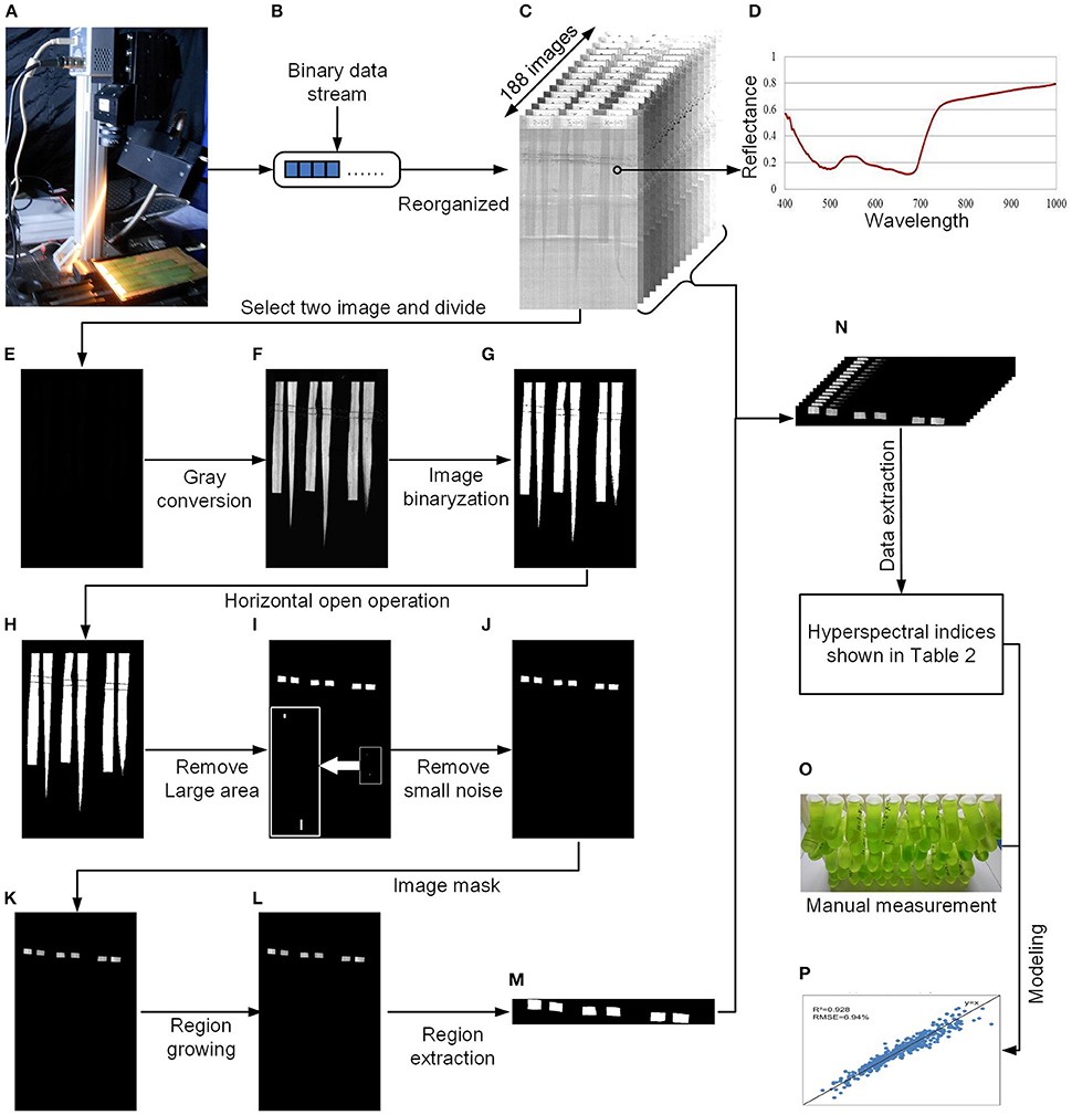
Figure 2. Flow chart of data processing. (A) System diagram. (B) Binary data stream acquired by the hyperspectral imaging system. (C) Hyperspectral images reorganized from the binary data stream. (D) Reflectance of the rice leaf. (E) Divided results (float image) of the two hyperspectral images. (F) Conversion of the float image to 8-bit grayscale. (G) Image binarization. (H) Horizontal open operation. (I) Removal of the large area. (J) Removal of small noise. (K) Image masking. (L) Region growing. (M) Region extraction. (N) All extractive images. (O) Manual measurement of the pigments. (P) Modeling and validation.
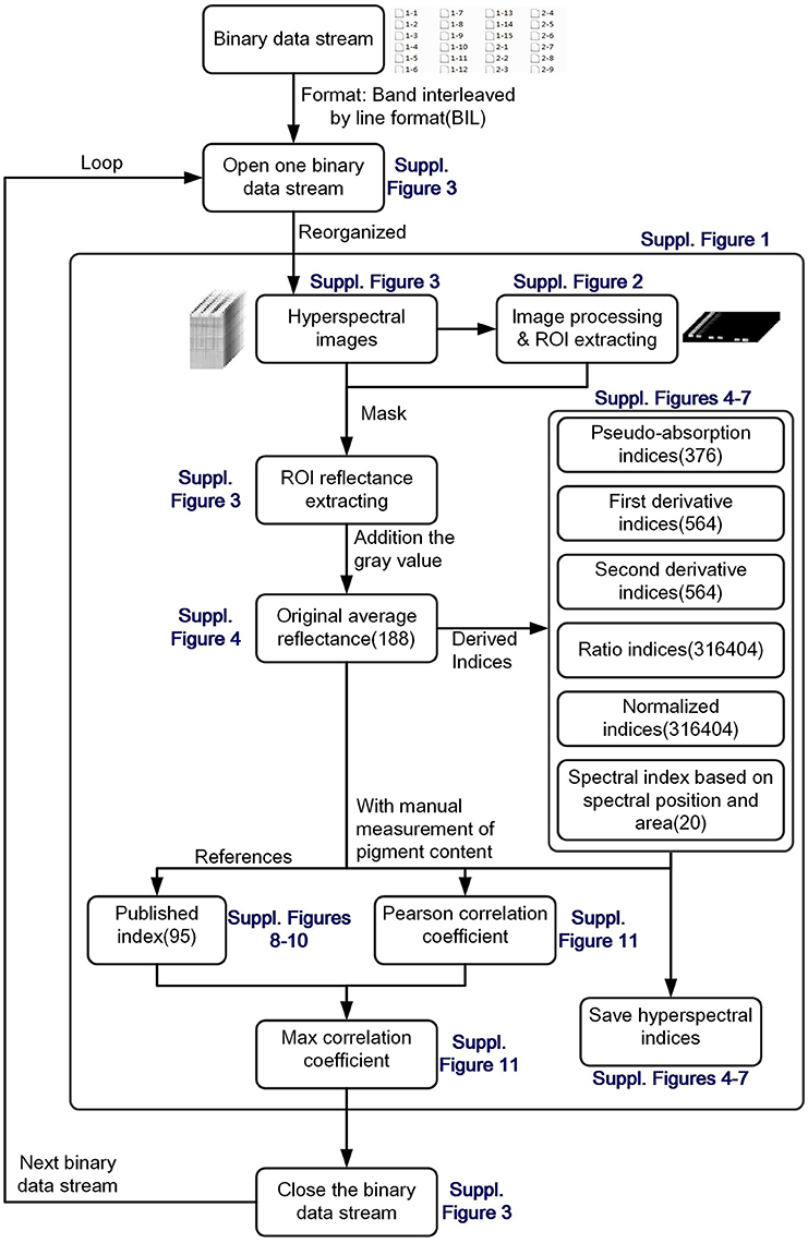
Figure 3. Flow chart of integrated hyperspectral image analysis pipeline.
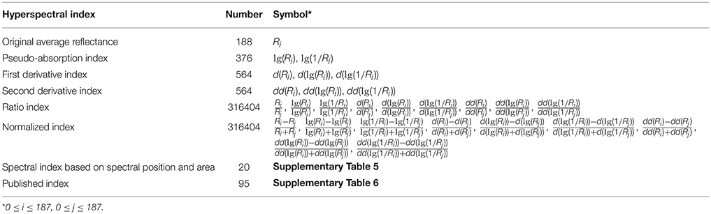
Table 2. Table 2 Definition and calculation formulas of 634,615 hyperspectral indices.
Manual Measurement
After hyperspectral imaging system acquisition, the ROI of each leaf was immersed in a 95% ethanol solution. When all of the pigments had been dissolved, a spectrophotometer (L3, INESA, China) was used to measure the absorbance values of the solution at different wavelengths (470, 649, and 665 nm, Figure 2O). Finally, the contents of 4 pigments, chlorophyll a, chlorophyll b, carotenoid, and total chlorophyll, were calculated according to Equations (1)–(4) (Arnon, 1949).
Ca is the chlorophyll a content, Cb is the chlorophyll b content, Cxc is the carotenoid content, and C is the total chlorophyll content. A665, A649, and A470 represent the absorbance at 665, 649, and 470 nm, respectively.
The distribution of the pigments at the two stages of plant growth is shown in Supplementary Table 3. For instance, at the tillering stage, the chlorophyll a content ranged from 61.24 to 573.63 mg/m2. The average value, the standard deviation, and the variable coefficient were 294.35 mg/m2, 92.19 mg/m2, and 31.32%, respectively. The correlation coefficients (r) between the pigments for the two stages were all above 0.88 (Supplementary Table 4), demonstrating that the concentrations of the various pigments were highly correlated.
Data Analysis and Modeling
To determine the specific bands that are highly correlated with chlorophyll a, we calculated all of the correlation coefficients between 634,615 spectral indices and 4 pigments. The calculation of correlation coefficients was programmed using LabVIEW 8.6 (National Instruments, Inc., USA). The hot bands were found using the heat maps of the correlation coefficients, which were drawn using HemI software (Deng et al., 2014). After all of the indices were obtained, the best index with the highest r was identified and used to build 5 models (linear, power, exponential, logarithmic, and quadratic models). The statistical analyses of the 5 models (linear, power, exponential, logarithm, and quadratic model) for 4 pigments and cross-validation were implemented with LabVIEW 8.6 (National Instruments, Inc., USA). To evaluate the model performance with primary indices or multiple variables, stepwise regression analysis (SRA) was conducted using SPSS software (Statistical Product and Service Solutions, Version 13.0, SPSS Inc., USA) (Figure 2P). Finally, the digitization of pigment distribution was performed using LabVIEW 8.6 (National Instruments, Inc., USA).
Results and Discussion
The Relationship between Chlorophyll a Concentration and Hyperspectral Indices
The number of total indices was too large to handle (634,615 indices for each sample); thus, to decrease the number of redundant indices, we first determined the relationship between the chlorophyll content and all the hyperspectral indices. Because the pigments were highly correlated with each other (Supplementary Table 4), we used chlorophyll a as an example to define the relationship between the pigments and the hyperspectral indices. In the 500–700 nm region (Figure 4A), the reflectance R was inversely correlated with the chlorophyll a content, indicating that the higher the reflectance was, the lower the chlorophyll a content was. This occurred because leaves with high chlorophyll content absorbed more light, causing the reflectance to decrease (Figure 2D). From Figures 4A–F, we found that compared with a logarithmic transformation, the use of derivative transformations such as dR, ddR, d(lg(1/R)), and dd(lg(1/R)) could provide more abundant hyperspectral information.
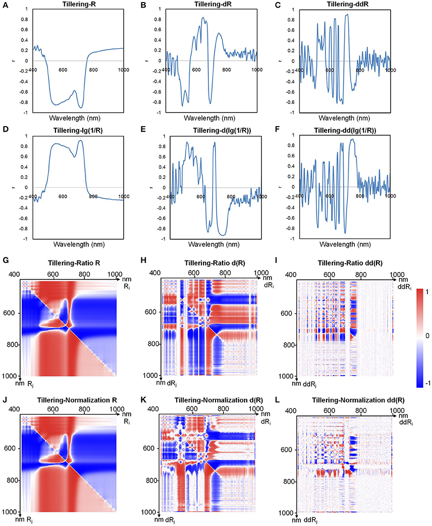
Figure 4. Correlation coefficients between chlorophyll a and (A) R, (B) dR, (C) ddR, (D) lg(1/R), (E) d(lg(1/R)), (F) dd(lg(1/R)), (G) ratio R, (H) ratio dR, (I) ratio ddR, (J) normalization R, (K) normalization dR, and (L) normalization ddR at the tillering stage.
Figures 4G–I show the correlation between the ratio index as defined in Table 2 and chlorophyll a, and Figures 4J–L show the correlation between the normalized index (also defined in Table 2) and chlorophyll a. Each point on the heat map represents the correlation coefficient between a hyperspectral index and the chlorophyll a level. The correlation coefficients for other indices and the chlorophyll a level are shown in Supplementary Figures 12, 13. When Ri and Rj were both in the 500–750 nm region, the correlation coefficient was high, sometimes even close to 1. Thus, we can infer that useful information for estimating chlorophyll a can be obtained in the wavelength range 500–750 nm.
By comparing the data shown in Figures 4G–I, we found that for the ratio indices, the correlation between the derivative indices and chlorophyll a decreased, and the original hyperspectral index (average reflectance, R) showed better correlation with chlorophylla. As illustrated in Figures 4J–L, the same results could be obtained for the normalized indices. Thus, to decrease the redundant indices, primary indices, including the original average reflectance (Ri), first derivative index (d(Ri)), second derivative index (dd(Ri)), ratio index (Ri/Rj), and normalized index ((Ri-Rj)/(Ri+Rj)), were used for the subsequent modeling and prediction of chlorophyll levels. A combined heat map obtained by adding together all of the heat maps of ratio and normalization coefficients is shown in Figure 5. From this, we found that the region of the highest correlation was located between 700 and 760 nm. If only the primary indices in the 700–760 nm region were used, the number of indices would decrease from 634, 615 to 483.
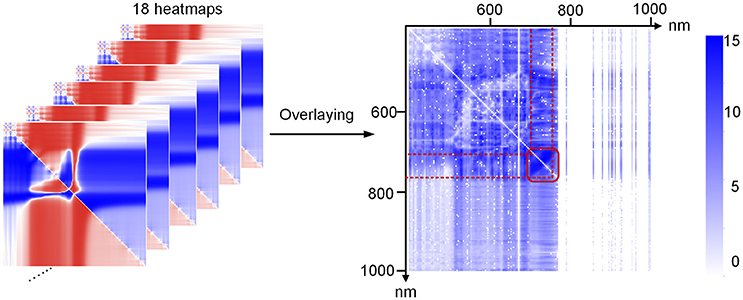
Figure 5. Summed coefficient image of all of the ratio and normalization coefficient images.
Linear Modeling with a Single Variable
After all of the indices were calculated, the hyperspectral indices with the highest correlation coefficients (r) of the pigments were selected for the modeling step, as shown in Table 3. The single-variable model for 4 pigments at the tillering and heading stages is shown in Table 4, which show that R2 ranged from 0.654 to 0.928, and the mean absolute percentage error (MAPE) was 6.94–12.84%. The scatter plots and the distribution of the relative error are shown in Figure 6 and Supplementary Figure 14, respectively, which show the points to be evenly distributed around the line y = x and that most of the relative error within the range ±10%. A 5-fold cross-validation of the single variable model for the 4 pigments at the two stages is shown in Table 4, which shows the ranges of R2 and MAPE as 0.671–0.930 and 7.49–13.02%, respectively.
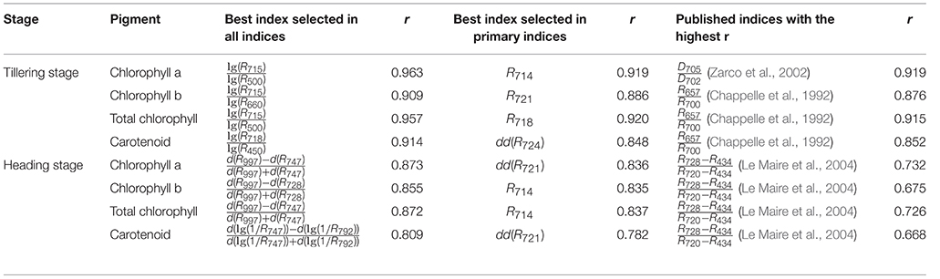
Table 3. Hyperspectral indices that displayed the highest r values selected from all indices or primary indices for the 4 pigments and comparison with published indices.
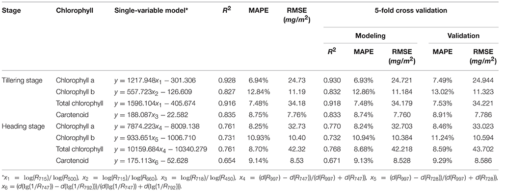
Table 4. Details of the single-variable models for the 4 pigments.
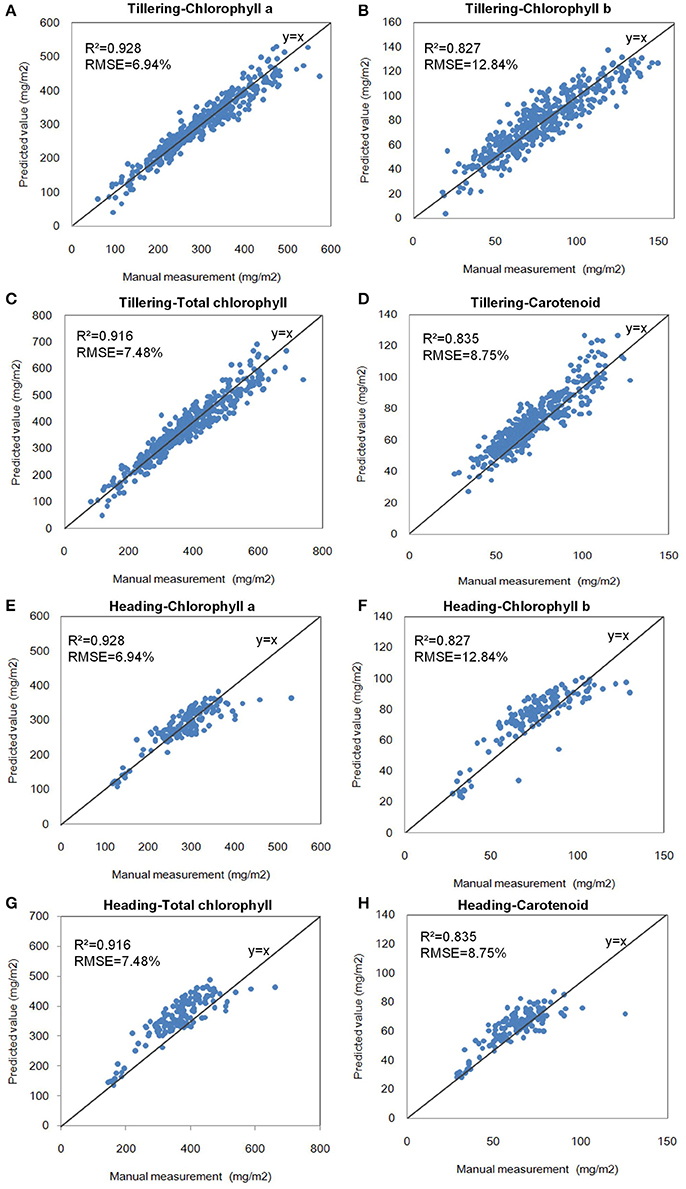
Figure 6. Scatter plots of the single-variable model of pigments at the two stages. (A) Chlorophyll a at the tillering stage. (B) Chlorophyll b at the tillering stage. (C) Total chlorophyll at the tillering stage. (D) Carotenoid at the tillering stage. (E) Chlorophyll a at the heading stage. (F) Chlorophyll b at the heading stage. (G) Total chlorophyll at the heading stage. (H) Carotenoid at the heading stage.
To evaluate the model's robustness, we evaluated the relationship between lg(R715)/lg(R500) and the chlorophyll a level for different accessions grown under different nitrogen regimes at the tillering stage (Figure 7). The model was not sensitive to accession or the nitrogen application level. Figure 7B shows that the amount of chlorophyll an increased with increase in the nitrogen application level. Moreover, we also compared the best model for the 4 pigments in this study with the published indices, as shown in Table 3 and Supplementary Table 6. The correlation between the pigments and the indices selected in this study (0.81–0.96) was higher than the correlation between the pigments and the published index with the highest r (0.67–0.92). On the other hand, all of the published indices with high r values were based on at least one wavelength in the range of 700–760 nm, implying that this range (700–760 nm) is important for the quantification of leaf chlorophyll.
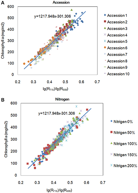
Figure 7. Relationship between R715/R500 and chlorophyll a content for different accessions (A) and for the same accessions under different nitrogen application levels (B) at the tillering stage.
Comparison of Linear and Non-linear Models
To determine the best model for determination of chlorophyll a levels, 5 models, including the linear, power, exponential, logarithmic, and quadratic models, were compared. The results are shown in Table 5. We found that the linear model had the highest R2 (0.928) and lowest MAPE (6.94%). Based on the relative robustness of the models, the linear model was selected as the final model for the quantification of chlorophyll. The results also indicate that the best relationship between the chlorophyll content and the index value was linear in our study.
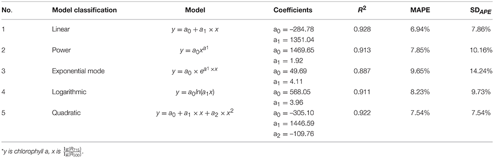
Table 5. Statistical summary of the 5 developed models for chlorophyll a estimation (sample size = 425)*.
Comparison of Models with All Indices and Models with Primary Indices
To compare the models that use all indices with those that use primary indices, we used 634,615 indices, and 483 primary indices for evaluating the model performance. The results (Table 3) showed that the highest r of the models that used primary indices (0.782–0.920) was similar to the highest r of the models that used all indices (0.809–0.963), indicating that the models that use primary indices are sufficiently accurate for the quantification of the 4 pigments. If only the primary indices were extracted and analyzed, the volume of hyperspectral data decreased from hundreds of thousands to hundreds, which dramatically reduced the workload of data acquisition and data analysis. The results of this comparison are shown in Table 3 and Supplementary Table 7.
Linear Modeling with Multi-Variables
We also evaluated the model performance using multi-variables. To faciliate the evaluation, only some primary indices, including R, dR, and ddR, were used to build the model using a stepwise regression analysis. The results (Supplementary Table 8) showed that R2 and Radj2 increased slightly and that MAPE and RMSE decreased slightly as the number of independent variables increased. The distribution of the relative error of the model using a stepwise regression analysis and multi-variables for chlorophyll a at the tillering stage is shown in Supplementary Figure 15, and 5-fold cross-validation of these models is shown in Supplementary Table 8.
Digitization of Leaf Chlorophyll Distribution
After the best single-variable model was built, it was used to digitize the leaf chlorophyll distribution at a high resolution (0.11 mm/pixel), as shown in Figure 8 (pseudo-color images). Figures 8A–C show the results obtained for one accession grown under different nitrogen application levels; with increasing nitrogen application, the chlorophyll a content increased dramatically. The chlorophyll a content of different accessions grown under the same nitrogen application level also varied (Figures 8D–F). Figures 8A–F show that for most samples, the chlorophyll concentration in the middle portion of the leaf was the highest, followed by the lower leaf and the upper leaf. Moreover, for the same leaf, the chlorophyll a content of the leaf vein was less than that of the leaf pulp, as shown in Figure 8G.
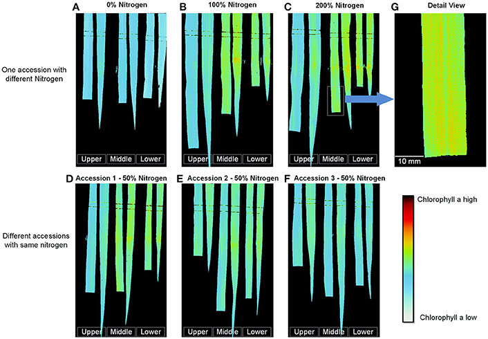
Figure 8. Digitization of the leaf chlorophyll distribution at the tillering stage. (A–C) One accession with different nitrogen application levels. (D–F) Different accessions with the same nitrogen application level. (G) Detailed image of (C). (To facilitate comparison, the gray stretching parameters of A–C were the same, and the gray stretching parameters of D–F were the same).
Modeling Nitrogen with Hyperspectral Imaging
A recent study showed that R2 between the total chlorophyll content and leaf nitrogen content of Papaya plants (Castro et al., 2011) could reach 0.78, and hyperspectral reflectance measurements could reflect the canopy nitrogen content of winter wheat (Zhou et al., 2016). To test the correlation between the nitrogen and hyperspectral indices in rice, we measured 90 rice accessions, selected from 533 rice core germplasm resources, using an auto discrete analyzer (Smartchen 200, France), SPAD-502, and hyperspectral imaging. The correlation coefficient (r) between the SPAD value and the nitrogen content was 0.766 (Figure 9A), and r between the nitrogen content and hyperspectral measurements with 4 indices was 0.897 (Figure 9B). Moreover, only using one index, the r between the nitrogen content and hyperspectral measurements was 0.773 (Figure 9C). The results showed that nitrogen in rice plants could also be quantified using hyperspectral imaging.
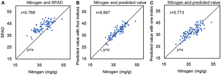
Figure 9. The correlation coefficient (r) between the SPAD value and the nitrogen content (A), between the nitrogen content and hyperspectral measurements with 4 indices (B), and between the nitrogen content and hyperspectral measurements with 1 index (C).
Comparison of Recent Related Studies for Quantifying Chlorophyll or Nitrogen Distribution
We compared the present research with recent related studies and found that several key wavelengths that reflect chlorophyll, such as cotton at 715 and 750 nm (Yi et al., 2014), winter wheat at 705 nm and the red edge (Zhou et al., 2016), and grass at 690–750 (Tong and He, 2017), were co-determined. Moreover, the commonly adopted tools, such as ENVI and SAS, handled enormous amounts of hyperspectral data, particularly image analysis, with difficulty. To relieve the bottleneck, we developed an integrated image analysis pipeline in this study. With a single variable, the measuring accuracy of chlorophyll, R2, ranged from 0.654 to 0.928. Moreover, due to using hyperspectral imaging in a higher resolution (0.11 mm/pixel), the distribution of leaf chlorophyll could be clearly visualized. The goal of this article was to quantify the chlorophylls in individual rice leaves, which should be tested and verified in the field in future. Combining the current field phenotyping tools, such as field phenotyping at the plot level (Andrade-Sanchez et al., 2014) and movable imaging chambers in the field (Busemeyer et al., 2013), the integrated image analysis pipeline could be expanded to the field. Moreover, combined hyperspectral imaging with a novel sensor for structure imaging, such as a micro-CT (Mineyuki, 2014) and 3D laser scanning (Paulus et al., 2014), could also reconstruct the 3D distribution of chlorophyll in a high resolution.
Conclusions
In this study, we used a hyperspectral imaging system to develop an integrated image analysis pipeline to handle extremely large amounts of hyperspectral data automatically. We also built models that could be used to accurately quantify 4 rice leaf pigments and identify the important spectral bands (700–760 nm) associated with these pigments. Moreover, by combining the hyperspectral data and these models, the distribution of chlorophyll could be digitized with high resolution (0.11 mm/pixel). In the future, the pipeline and selected models can potentially be applied to quantify the chlorophyll distribution in individual plants non-destructively. Evidence from related works shows that the image analysis pipeline combined with hyperspectral imaging could also be extended for co-determining wavelengths for quantifying chlorophyll in other crops.
Author Contributors
HF and WY designed the research, performed the experiments, analyzed the data and wrote the manuscript. GC provided the rice samples and also performed experiments. LX and QL supervised the project, designed the research, and wrote the manuscript.
Conflict of Interest Statement
The authors declare that the research was conducted in the absence of any commercial or financial relationships that could be construed as a potential conflict of interest.
The reviewer RJW and handling Editor declared their shared affiliation, and the handling Editor states that the process met the standards of a fair and objective review.
Acknowledgments
This work was supported by grants from the National Program on High Technology Development (2013AA102403), the National key research and development program (2016YFD0100101-18), the Scientific Conditions and Resources Research Program of Hubei Province of China (2015BCE044), the China Postdoctoral Science Foundation (2016M592345), and the Fundamental Research Funds for the Central Universities (2662017PY058).
Supplementary Material
The Supplementary Material for this article can be found online at: http://journal.frontiersin.org/article/10.3389/fpls.2017.01238/full#supplementary-material
Supplementary Figure 1. Flow chart of the program. The number represents the processing module of the following Supplementary Figures 2–11.
Supplementary Figure 2. Program for image processing and ROI extraction. (A) Reorganized two images from the binary data stream (1), (B) Segment the leaf part from the background with the two images (2), (C) Image processing for the ROI extraction from the leaf part (3), (D) ROI extraction and save (4).
Supplementary Figure 3. Program for ROI reflectance extraction. (A) The main program for ROI reflectance extraction of all samples (5), (B) Creating the Excel file (6), (C) Savin the Excel file (7), (D) The sub-program for ROI reflectance extraction of single sample (8), (E) Applying the Supplementary Figure 2 results to the current data processing (9).
Supplementary Figure 4. Program for calculation of the original average reflectance (A) (10) and the spectral index based on spectral position and area (B) (11).
Supplementary Figure 5. Program for calculation of the first and second derivatives (12).
Supplementary Figure 6. Program for calculation of the pseudo-absorption index. (A) The calculation of the lgR (13), (B) The calculation of the lg(1/R) (14).
Supplementary Figure 7. Program for calculation of the ratio index. (A) The calculation of the 0-61 part of the ratio index (15), (B) The calculation of the 62–121 part of the ratio index (16), (C) The calculation of the 122–187 part of the ratio index (17). The programs for calculation of the normalized index are similar, except the Ri/Rj was changed into (Ri–Rj)/(Ri+Rj).
Supplementary Figure 8. Program for calculation of the partial published index. (A) Published index 1–3 (18), (B) Published index 4–9 (19), (C) Published index 10–15 (20), (D) Published index 16–22 (21).
Supplementary Figure 9. Program for calculation of the partial published index. (A) Published index 23–31 (22), (B) Published index 32–35 (23), (C) Published index 36–43 (24), (D) Published index 44–56 (25).
Supplementary Figure 10. Program for calculation of the partial published index. (A) Published index 57–67 (26), (B) Published index 68–79 (27), (C) Published index 80–85 (28), (D) Published index 86–95 (29).
Supplementary Figure 11. Program for calculation of the correlation coefficient. (A) The program for calculation of the correlation coefficients between all the pigments and all the hyperspectral indices (30), (B) The program for combination the correlation coefficients of the ratio and normalized indices (31), (C) The program for building image with the correlation coefficients (32), (D) The program for finding the max correlation coefficient (33).
Supplementary Figure 12. Correlation coefficients between chlorophyll a and ratio lg(R) (A), normalization lg(R) (B), ratio d(lg(R)) (C), normalization d(lg(R)) (D), ratio dd(lg(R)) (E), and normalization dd(lg(R)), (F) at the tillering stage.
Supplementary Figure 13. Correlation coefficients between chlorophyll a and ratio lg(1/R) (A), normalization lg(1/R) (B), ratio d(lg(1/R)) (C), normalization d(lg(1/R)) (D), ratio dd(lg(1/R)) (E), and normalization dd(lg(1/R)) (F) at the tillering stage.
Supplementary Figure 14. Distribution of relative error of the single-variable models for the chlorophyll a (A), chlorophyll b (B), total chlorophyll (C), and carotenoid (D) at the tillering stage. Distribution of relative error of the single-variable models for the chlorophyll a (E), chlorophyll b (F), total chlorophyll (G), and carotenoid (H) at the heading stage.
Supplementary Figure 15. Distribution of relative error of the one independent variable (A), two independent variables (B), three independent variables (C), four independent variables (D) models using stepwise regression analysis for chlorophyll a at the tillering stage.
Supplementary Table 1. The latest related papers of chlorophyll or nitrogen quantification with spectral methods.
Supplementary Table 2. Information about the 90 rice accessions and SPAD value.
Supplementary Table 3. Distribution of the pigments at the two stages.
Supplementary Table 4. Correlation coefficient (r) between the pigments at the two stages.
Supplementary Table 5. Spectral index based on spectral position and area.
Supplementary Table 6. Published spectral indices∗.
Supplementary Table 7. Comparison of performance between models using all of the indices and models using original indices.
Supplementary Table 8. Details of the multiple-variable models for 4 pigments.
References
Andrade-Sanchez, P., Gore, M. A., Heun, J. T., Thorp, K. R., Carmo-Silva, A. E., French, A. N., et al. (2014). Development and evaluation of a field-based high-throughput phenotyping platform. Funct. Plant Biol. 41, 68–79. doi: 10.1071/FP13126
Arnon, D. I. (1949). Copper enzymes in isolated chloroplasts: polyphenoloxidase in Beta vulgaris. Plant Physiol. 24, 1–15. doi: 10.1104/pp.24.1.1
Baret, F., Jacquemoud, S., Guyot, G., and Leprieur, C. (1992). Modeled analysis of the biophysical nature of spectral shifts and comparison with information content of broad bands. Remote Sens. Environ. 41, 133–142. doi: 10.1016/0034-4257(92)90073-S
Benedict, H., and Swidler, R. (1961). Nondestructive method for estimating chlorophyll content of leaves. Science 133, 2015–2016. doi: 10.1126/science.133.3469.2015
Blackburn, G. (1998a). Quantifying chlorophylls and caroteniods at leaf and canopy scales: an evaluation of some hyperspectral approaches. Remote Sens. Environ. 66, 273–285. doi: 10.1016/S0034-4257(98)00059-5
Blackburn, G. (1998b). Spectral indices for estimating photosynthetic pigment concentrations: a test using senescent tree leaves. Int. J. Remote Sens. 19, 657–675. doi: 10.1080/014311698215919
Blackburn, G., and Pitman, J. (1999). Biophysical controls on the directional spectral reflectance properties of bracken (Pteridium aquilinum) canopies: results of a field experiment. Int. J. Remote Sens. 20, 2265–2282. doi: 10.1080/014311699212245
Busemeyer, L., Ruckelshausen, A., Moeller, K., Melchinger, A. E., Alheit, K. V., Maurer, H. P., et al. (2013). Precision phenotyping of biomass accumulation in triticale reveals temporal genetic patterns of regulation. Sci. Rep. 3:2442. doi: 10.1038/srep02442
Carter, G. A. (1998). Reflectance wavebands and indices for remote estimation of photosynthesis and stomatal conductance in pine canopies. Remote Sens. Environ. 63, 61–72. doi: 10.1016/S0034-4257(97)00110-7
Castro, F. A., Campostrini, E., Netto, A. T., and Viana, L. H. (2011). Relationship between photochemical efficiency (JIP-Test Parameters) and portable chlorophyll meter readings in papaya plants. Braz. J. Plant Physiol. 23, 295–304. doi: 10.1590/S1677-04202011000400007
Chappelle, E., Kim, M., and Mcmurtrey, J. (1992). Ratio analysis of reflectance spectra (RARS): an algorithm for the remote estimation of the concentrations of chlorophyll a, chlorophyll b, and carotenoids in soybean leaves. Remote Sens. Environ. 39, 239–247. doi: 10.1016/0034-4257(92)90089-3
Deng, W., Wang, Y., Liu, Z., Cheng, H., and Xue, Y. (2014). HemI: a toolkit for illustrating heatmaps. PLoS ONE 9:e111988. doi: 10.1371/journal.pone.0111988
Ergun, E., Demirata, B., Gumus, G., and Apak, R. (2004). Simultaneous determination of chlorophyll a and chlorophyll b by derivative spectrophotometry. Anal. Bioanal. Chem. 379, 803–811. doi: 10.1007/s00216-004-2637-7
Gamon, J., and Surfus, J. (1999). Assessing leaf pigment content and activity with a reflectometer. New Phytol. 143, 105–117. doi: 10.1046/j.1469-8137.1999.00424.x
Jasinski, S., Lécureuil, A., Durandet, M., Bernard-Moulin, P., and Guerche, P. (2016). Arabidopsis seed content qtl mapping using high-throughput phenotyping: the assets of near infrared spectroscopy. Front. Plant Sci. 7:1682. doi: 10.3389/fpls.2016.01682
Kochubey, S., and Kazantsev, T. (2007). Changes in the first derivatives of leaf reflectance spectra of various plants induced by variations of chlorophyll content. J. Plant Physiol. 164, 1648–1655. doi: 10.1016/j.jplph.2006.11.007
Le Maire, G., Francois, C., and Dufrene, E. (2004). Towards universal broad leaf chlorophyll indices using PROSPECT simulated database and hyperspectral reflectance measurements. Remote Sens. Environ. 89, 1–28. doi: 10.1016/j.rse.2003.09.004
Miller, J., Hare, E., and Wu, J. (1990). Quantitative characterization of the vegetation red edge reflectance 1. An inverted-Gaussian reflectance model. Remote Sens. 11, 1755–1773. doi: 10.1080/01431169008955128
Mineyuki, Y. (2014). 3D image analysis of plants using electron tomography and micro-CT. Microscopy 63(Suppl. 1), i8–i9. doi: 10.1093/jmicro/dfu036
Moharana, S., and Dutta, S. (2016). Spatial variability of chlorophyll and nitrogen content of rice from hyperspectral imagery. ISPRS J. Photogrammetry Remote Sens. 122, 17–29. doi: 10.1016/j.isprsjprs.2016.09.002
Montagnoli, A., Terzaghi, M., Fulgaro, N., Stoew, B., Wipenmyr, J., Ilver, D., et al. (2016). Non-destructive phenotypic analysis of early stage tree seedling growth using an automated stereovision imaging method. Front. Plant Sci. 7:1644. doi: 10.3389/fpls.2016.01644
Moss, D. M., and Rock, B. N. (1991). “Analysis of red edge spectral characteristics and total chlorophyll values for red spruce (Picea Rubens) branch segments from Mt. Moosilauke, NH, USA,” in Geoscience and Remote Sensing Symposium, (1991). IGARSS '91. Remote Sensing: Global Monitoring for Earth Management., International (Durham, NC), 1529–1532.
Narsai, R., Devenish, J., Castleden, I., Narsai, K., Xu, L., Shou, H., et al. (2013). Rice DB: an Oryza information portal linking annotation, subcellular location, function, expression, regulation, and evolutionary information for rice and Arabidopsis. Plant J. 76, 1057–1073. doi: 10.1111/tpj.12357
Negi, M., Sanagala, R., Rai, V., and Jain, A. (2016). Deciphering phosphate deficiency-mediated temporal effects on different root traits in rice grown in a modified hydroponic system. Front. Plant Sci. 7:550. doi: 10.3389/fpls.2016.00550
Paulus, S., Schumann, H., Kuhlmann, H., and Leon, J. (2014). High-precision laser scanning system for capturing 3D plant architecture and analysing growth of cereal plants. Biosyst. Eng. 121, 1–11. doi: 10.1016/j.biosystemseng.2014.01.010
Sievers, G., and Hynninen, P. H. (1977). Thin-layer chromatography of chlorophylls and their derivatives on cellulose layers. J. Chromatogr. 134, 359–364. doi: 10.1016/S0021-9673(00)88534-9
Sporer, A. H., Freed, S., and Sancier, K. M. (1954). Paper chromatography of chlorophylls. Science 119, 68–69. doi: 10.1126/science.119.3080.68
Thorp, K. R., Wang, G., Bronson, K. F., Badaruddin, M., and Mon, J. (2017). Hyperspectral data mining to identify relevant canopy spectral features for estimating durum wheat growth, nitrogen status, and grain yield. Comput. Electron. Agric. 136, 1–12. doi: 10.1016/j.compag.2017.02.024
Tong, A., and He, Y. (2017). Estimating and mapping chlorophyll content for a heterogeneous grassland: comparing prediction power of a suite of vegetation indices across scales between years. ISPRS J. Photogrammetry Remote Sens. 126, 146–167. doi: 10.1016/j.isprsjprs.2017.02.010
Xue, L., and Yang, L. (2009). Deriving leaf chlorophyll content of green-leafy vegetables from hyperspectral reflectance. ISPRS J. Photogram. Remote Sens. 64, 97–106. doi: 10.1016/j.isprsjprs.2008.06.002
Yang, W., Duan, L., Chen, G., Xiong, L., and Liu, Q. (2013). Plant phenomics and high-throughput phenotyping: accelerating rice functional genomics using multidisciplinary technologies. Curr. Opin. Plant Biol. 16, 180–187. doi: 10.1016/j.pbi.2013.03.005
Yi, Q., Jiapaer, G., Chen, J., Bao, A., and Wang, F. (2014). Different units of measurement of carotenoids estimation in cotton using hyperspectral indices and partial least square regression. ISPRS J. Photogram. Remote Sens. 91, 72–84. doi: 10.1016/j.isprsjprs.2014.01.004
Yuan, J., Zhang, Y., Shi, X., Gong, X., and Chen, F. (1997). Simultaneous determination of carotenoids and chlorophylls in algae by high performance liquid chromatography. Chin. J. Chromatogr. 15, 133–135.
Zarco, P., Miller, J., Mohammed, G., Noland, T., and Sampson, P. (2002). Vegetation stress detection through chlorophyll+ estimation and fluorescence effects on hyperspectral imagery. J. Environ. Qual. 31, 1433–1441. doi: 10.2134/jeq2002.1433
Zhang, Q. F. (2007). Strategies for developing green super rice. Proc. Natl. Acad. Sci. U.S.A. 104, 16402–16409. doi: 10.1073/pnas.0708013104
Zhou, X., Huang, W., Kong, W., Ye, H., Luo, J., and Chen, P. (2016). Remote estimation of canopy nitrogen content in winter wheat using airborne hyperspectral reflectance measurements. Adv. Space Res. 58, 1627–1637. doi: 10.1016/j.asr.2016.06.034
Keywords: chlorophyll, hyperspectral imaging, image analysis pipeline, rice, phenomics
Citation: Feng H, Chen G, Xiong L, Liu Q and Yang W (2017) Accurate Digitization of the Chlorophyll Distribution of Individual Rice Leaves Using Hyperspectral Imaging and an Integrated Image Analysis Pipeline. Front. Plant Sci. 8:1238. doi: 10.3389/fpls.2017.01238
Received: 30 November 2016; Accepted: 30 June 2017;
Published: 25 July 2017.
Edited by:
John Doonan, Aberystwyth University, United KingdomReviewed by:
Ming Chen, Zhejiang University, ChinaYuhui Chen, Noble Research Institute, LLC., United States
Richard John Webster, Aberystwyth University, United Kingdom
Copyright © 2017 Feng, Chen, Xiong, Liu and Yang. This is an open-access article distributed under the terms of the Creative Commons Attribution License (CC BY). The use, distribution or reproduction in other forums is permitted, provided the original author(s) or licensor are credited and that the original publication in this journal is cited, in accordance with accepted academic practice. No use, distribution or reproduction is permitted which does not comply with these terms.
*Correspondence: Qian Liu, cWlhbmxpdUBtYWlsLmh1c3QuZWR1LmNu
Wanneng Yang, eXduQG1haWwuaHphdS5lZHUuY24=